How to Use Named Ranges in Power Query

Power Query is a useful way to pull in data and make changes to it. The steps get recorded as you make them to your data set. But by doing so, you can also be hardcoding some of those steps along the way. That’s a no-no. When possible, you should make your formulas, macros, and templates as dynamic as possible. One way you can do that in Power Query is by using named ranges. In this post, I’ll show you how you to do that.

Start with creating a regular named range

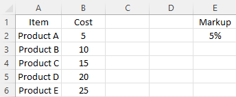
In this example, I’m going to use a named range to make it easy to change the markup on products. Here is a list of some generic products and prices:

In Cell E2, I have my markup percentage. I’m going to create a named range called ‘markup’ for this cell.

Assigning that named range in Power Query

Next, I’ll create a Power Query connection by selecting any of the values above in columns A or B. Under the Data tab, selecting From Table/Range under the Get & Transform Data section will launch Power Query. From that screen, you can launch the Advanced Editor under the Query section of the Home tab. That will open up a new window where the code is stored:

There is not a whole lot there right now just because the only thing I’ve done thus far is just link to the Excel table. Above the Source line, I’m going to add my named range. I’ll call this Markup as well. The formula to reference my cell is as follows:

Markup = Excel.CurrentWorkbook(){[Name="markup"]}[Content]{0}[Column1]

As you can see the named range of ‘markup’ is referenced and it’s important it is spelled exactly the same way as the code in Power Query is case-sensitive. The above code creates a table and by referencing {0}[Column1] I’m directing it to the value in the first row, and first column. It’s an important part of the code, otherwise, you will get something that Power Query doesn’t recognize as being a single value. Add the above line, along with a comma after it in the code. Here’s how it should look:

When I close out of that and go back into the main Power Query window, there’s a new step called Markup where I’ve assigned my named range. Now all that’s left is to do something with this named range.

Create a custom column to use a named range in a calculation

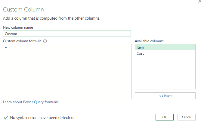
On the Add Column tab in Power Query, there’s an option to create a Custom Column. If you click on that, you’ll see the following window, where you can create a formula:

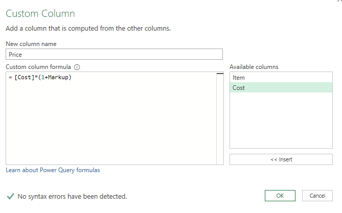
You can double-click the available columns off on the right to insert them into the formula. This will be a fairly straightforward formula where I’ll take the cost and multiply it by 1 plus the Markup variable I created earlier:

Now a new column has been created:

And that’s it. Now I can hit Close & Load to get back into the worksheet, where I’ll now have a price column. Changing the markup value in the sheet and then refreshing the data will update the price column to reflect the new markup percentage.

If you liked this post on How to Use Named Ranges in Power Query, please give this site a like on Facebook and also be sure to check out some of the many templates that we have available for download. You can also follow us on Twitter and YouTube.