
The default pivot table layout can oftentimes be suboptimal. The compact view doesn’t make it easy for analyzing data, especially when you have many fields. If you’re like me, one of the first things you probably do after creating a pivot table is to change the layout so it’s easier to view the data. The good news is you don’t have to keep repeating those steps. You can change the default so that when you create a pivot table, it’ll already have your desired settings applied. In this post, I’ll show you how to do that.
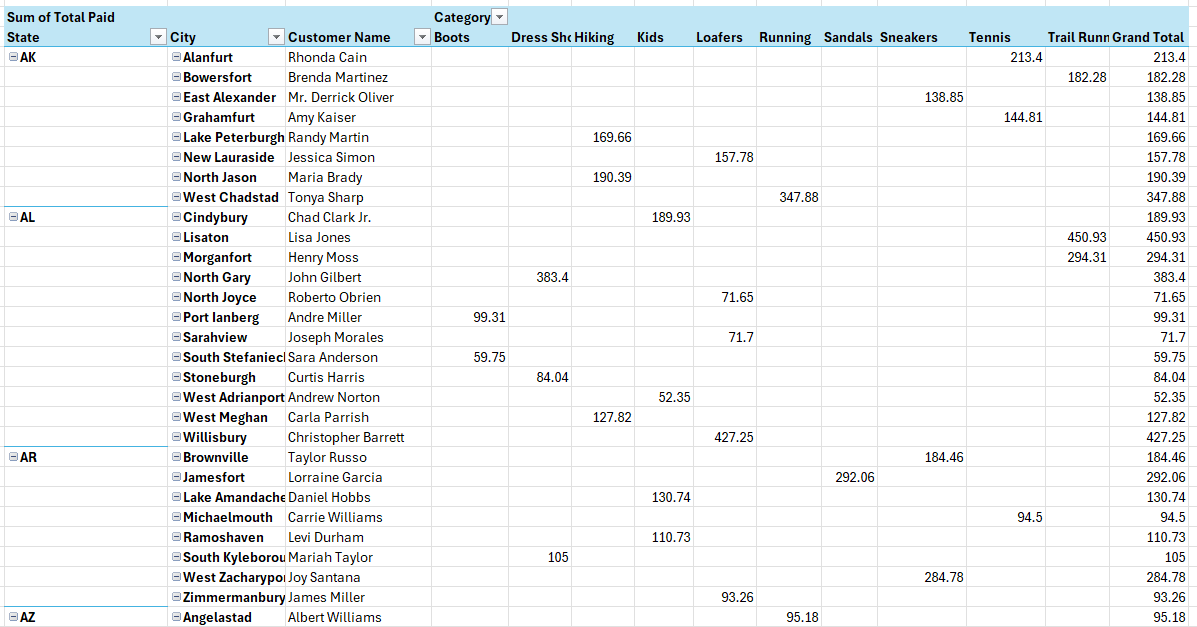
Here’s a sample pivot table, which shows you sales broken out by city, state, customer, and in this case, the type of product (shoe) sold:
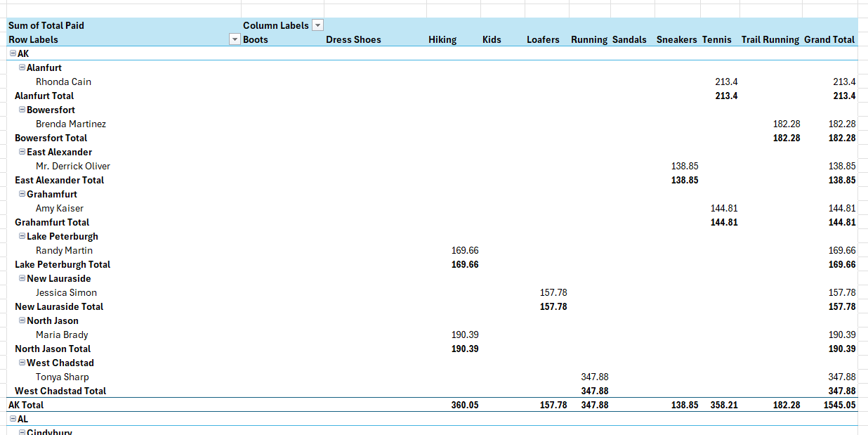
There are many things which are suboptimal here, including the following:
- The compact format has put the customer, city, and state fields all in the same column.
- There are many subtotals, which create repeating values in this data set and are unnecessary.
To start, I’ll make these changes manually and then save those options as my default.
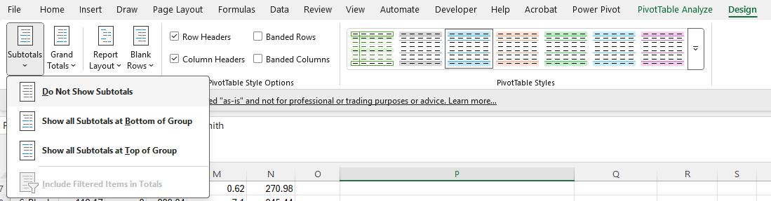
To turn off subtotals, I can go into the Design tab (the pivot table has to be selected for this to be visible) and under Subtotals, select the option to not show subtotals:
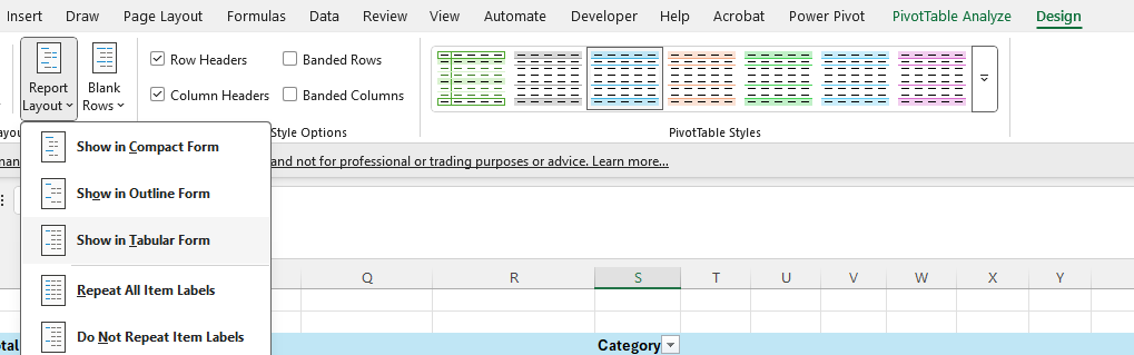
To change the layout from compact, I’ll stay in the Design tab and select Report Layout and choose Show in Tabular Form.
This now produces the following pivot table:
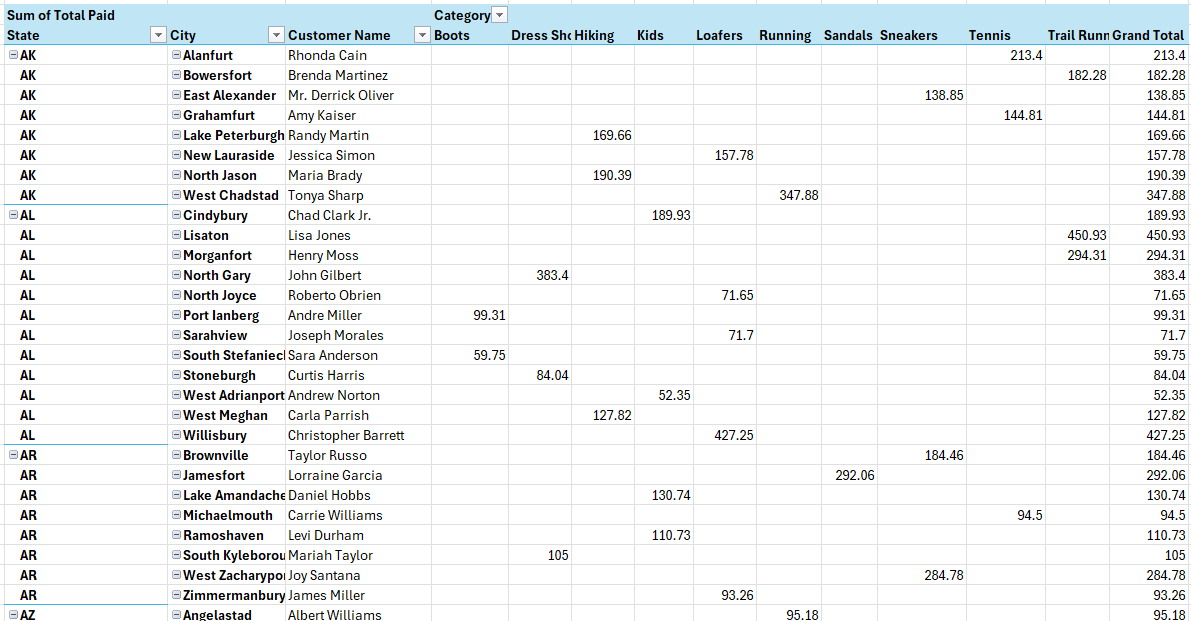
This, however, is still not ideal as the state values only appear once. Instead, I’d like to see the value repeating so that every line has every field filled in. This makes it ideal if you want to use any formulas that reference the pivot table. Back in the Report Layout section, there is an option to select Repeat All Item Labels. Upon doing this, now my pivot table is filled in for all possible fields:
This is how I prefer to setup my pivot table. But rather than having to repeat the process each time, I can save these settings.
How to save your preferred pivot table layout as the default
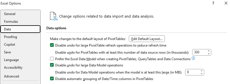
To save your preferred layout (after setting it up), go into the File tab and select Options at the bottom, which will open up the Excel Options. And if you navigate to the Data section, you will see the first option relates to the default layout of Pivot Tables — click the button to Edit Default Layout.
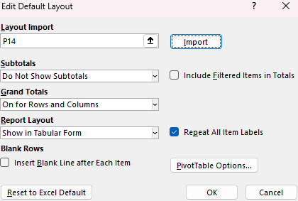
Next, you’ll find all the different options you can specify for your pivot table:
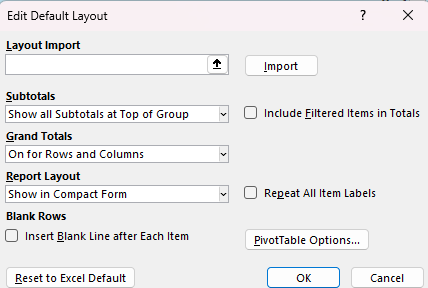
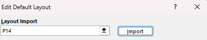
You can specify these different settings for subtotals, grand totals, and labels. Or, what you can also do is import the layout. To do this, simply click on a cell in your pivot table, and then click on the Import button. In my example, cell P14 contains my pivot table:
After clicking the Import button, the settings are automatically applied and updated:
As you can see, it has applied the changes for me, without having to make the changes manually from the different boxes and drop downs. This can be helpful if you’ve already setup a pivot table the way you want, rather than determining which different settings you want to apply. When you click on OK, now your settings will be applied.
The next time you create a pivot table, these saved settings will be in place and you won’t have to change them again. These settings are saved to your computer and even if you open a new Excel file and create a new pivot table, they will take effect.
If you liked this post on How to Change the Default Layout of Your Pivot Table in Excel, please give this site a like on Facebook and also be sure to check out some of the many templates that we have available for download. You can also follow me on Twitter and YouTube. Also, please consider buying me a coffee if you find my website helpful and would like to support it.