How to Use a Custom Number Format in Excel

There are many different options for formatting data in a spreadsheet. And there are even more available if you use a custom number format in Excel. That flexibility is important because it can be a bit frustrating if, for example, you want negative numbers to show up with a dollar sign as you have to use the currency format in that situation — which does not look very polished:

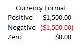
The positive and negative amounts look okay but I’d like to see a bit more spacing. But the bigger issue for me is the $0.00 formatting which can create a lot of noise if you’re looking at financials with lots of zeroes over the place (although I have a solution for this). It can divert your attention away from what you want to see — the cells that have non-zero values.

Creating a Custom Number Format

Although it may not be available by default, there is certainly a way to get a whole lot closer to the formatting that I want, and I’ll show you how. To start, you want to select the accounting format and then flip over to the Custom format (to do this right-click and select Format Cells). You’ll notice this is what the string looks like in the Type field:

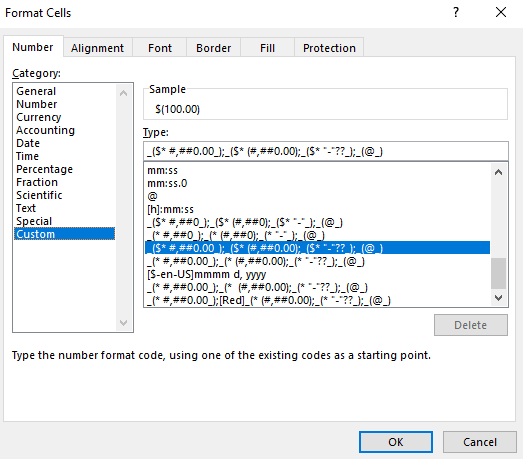
This is what the accounting format looks like. The formatting is broken out into four main parts: positive, negative, zero, and text.

The string that appears until the first semi-colon is how the number will look when it is positive. Until the next semi-colon is the negative formatting, followed by if the value is zero and the last one is text.

Here is what the positive amount looks like in the accounting format:

_($* #,##0.00);(

The negative formatting looks very similar:

_($* (#,##0.00);

The main difference you’ll notice is the extra bracket “(” that is in the negative format. That is what puts the negative amounts in parentheses. Now, if I want to make this highlighted in red, all I would need to do is add [Red] right after the semicolon that indicates the end of the positive format:

($* #,##0.00);[Red]($* (#,##0.00);($* “-“??);(@_)

Upon doing that change, my number now comes up in red:

These are all the color options you can use:

• Black
• Blue
• Cyan
• Green
• Magenta
• Red
• White
• Yellow

There’s not any added customization you can do to these colors. And as you can imagine, many of these colors will be an eyesore on the default white background, and I’m not sure why you would even need to use the default black value. Blue, magenta, and red are the only ones that are easy to read and that won’t make you want to change the background color.

More Customization Options

For more complete customization, you’re better off looking at how to use conditional formatting.

If you need to make other tweaks to number formats what you can do is select the format and then switch over to the Custom section. Then you’ll see what that format looks like and you can test out what adjustments you’d like. Whether it’s adjusting the spacing or how the format looks like with a zero value, these are changes you can easily make and see what works through some trial and error.

If you’re interested in looking how to format dates, check out this post.

If you liked this How to Create a Custom Number Format in Excel, please give this site a like on Facebook and also be sure to check out some of the many templates that we have available for download. You can also follow us on Twitter and YouTube.