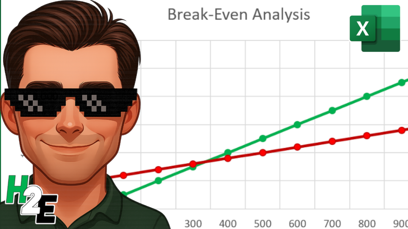
Every business owner, financial analyst, and student asks the same fundamental question: “How much do I need to sell to cover my costs?”
This is what your break-even point would be. It is where your total revenue equals your total costs, yielding zero profit, but also zero loss. This is a crucial number because you know if you produce more than what’s needed to hit break even, you’ll be turning a profit. Calculating this manually can be time-consuming, but building a dynamic break-even analysis in Excel can enable you to test different pricing strategies and cost structures instantly. In this guide, I’ll walk you through the process, the formulas, and how to visualize the data using Excel charts.
What is a Break-Even Analysis?
Before opening Excel, it is crucial to understand the three components that make up the break-even calculation:
- Fixed Costs: Expenses that stay the same regardless of how much you sell (e.g., rent, insurance, salaries).
- Variable Costs: Expenses that increase with every unit sold (e.g., raw materials, shipping, packaging).
- Selling Price: The amount you charge for one unit of your product.
The formula to find the number of units you need to sell to break even is:
Break-Even Units = Fixed Costs/(Selling Price - Variable Cost per Unit)
The denominator (Selling Price – Variable Cost) is also called the Contribution Margin. It represents how much money is left over from each sale to contribute toward paying off your fixed costs. If your contribution margin is not positive, then you’ll never been able to hit your break-even point.
Now that we understand the terms and key formulas, we can move on to setting up the break-even calculation in Excel.
Step 1: Set Up Your Data Table
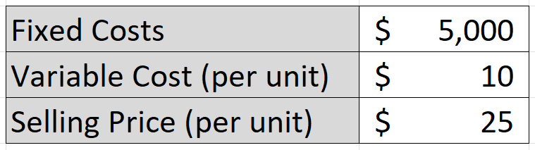
First, we need to input our variables. Open a new Excel sheet and create a distinct input area. This makes it easy to change numbers later without breaking your formulas.
Let’s pretend we are running a specialized T-shirt business, with the following costs and selling prices:
Step 2: Calculate the Break-Even Point
Now, let’s calculate the exact number of T-shirts we need to sell to cover that $5,000 in fixed costs. Using the aforementioned formula where we take the fixed costs and divide them by the contribution margin (selling price less variable cost), this results in the following calculation:

The formula in cell C6 is as follows:
=ROUNDUP(C2/(C4-C3),0)
The result is 333.33 units, but that ROUNDUP function rounds the result up to the nearest whole number, which is 334. Since you can’t sell a portion of a shirt, it’s necessary to round up.
Step 3: Create a Dynamic Data Model
Knowing the break-even point is helpful, but seeing the trend can be much more useful. Let’s create a table that calculates revenue and costs at different volume levels (e.g., selling 0 units, 100 units, 200 units, etc.).
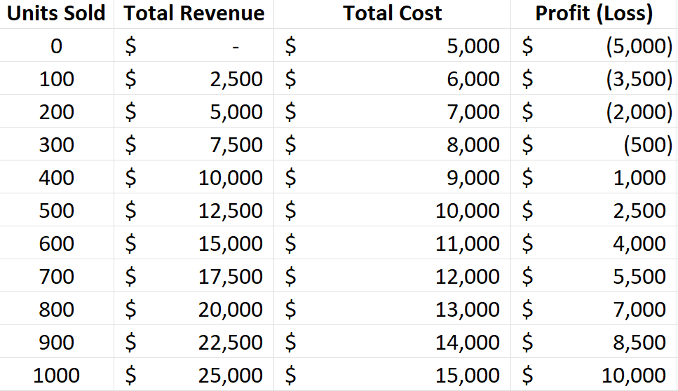
I’m going to set up a table with headers for the following fields: Units Sold, Total Revenue, Total Cost, and Profit (Loss). For Units Sold, the units will start from 0 and increment by 100 at a time. The Total Revenue field will multiply the units sold by the selling price. The Total Cost field will be equal to the units sold multiplied by the variable cost, with the fixed costs added on top. The Profit (Loss) will take the Total Revenue and deduct the Total Cost.
The table should look something like this:
Step 4: Visualize with a Break-Even Chart
Visuals make financial data easier to understand. We can create a chart that shows where the Total Revenue line crosses the Total Costs line.
To do this, start by highlighting three columns in your data table: Units Sold, Total Revenue, and Total Costs. Go to the Insert tab, open up the Charts window, and select any Line Chart you wish to use. You’ll need to adjust the data so that the Horizontal Axis Label for the Revenue and Cost fields is the Units Sold column.
You should now see a chart that looks similar to this:

As per the earlier analysis, we can see that the break-even point is right around 300 units, which is what the chart above indicates.
Step 5: Advanced Tip: Use Goal Seek to do a What-If Analysis
What if you don’t just want to break even? What if you want to make exactly $2,000 in profit this month? You can use Excel’s Goal Seek feature rather than guessing. In the following example, I’ve setup a couple of extra cells for units sold and one for profit (loss), which will be used in the goal seek calculation:

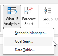
Now, let’s go to the Data tab, select What-If Analysis (under the Forecast section), and click on Goal Seek.
Based on the table above, let’s input the following values for the Goal Seek inputs:

The Set cell value is the ending value that we want, which in this case is the Profit (Loss) value, which is determined by selling price, variable cost, and fixed costs. We want this value to equal 2000, by changing cell C8, which is the number of units sold. After clicking OK, Goal Seeks does the work to figure out what the value in C8 needs to be for C9 to be equal to 2000.
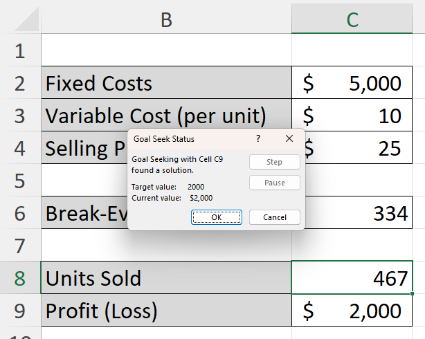
By clicking on OK, you’ll accept the results and they’ll remain in your table. This calculation tells me that by selling approximately 467 units, the profit will be $2,000.
If you liked this post on How to Calculate Break-Even Analysis in Excel: A Step-by-Step Guide, please give this site a like on Facebook and also be sure to check out some of the many templates that we have available for download. You can also follow me on X and YouTube. Also, please consider buying me a coffee if you find my website helpful and would like to support it.