dates – HowtoExcel.net

Adding Static Timestamps in Excel Using Checkboxes

March 26, 2024

by howtoexcel checkboxes circular reference data entry dates

One way to enhance your spreadsheets is by adding checkboxes. Using checkboxes, you can make data entry easier for your users. And you can create formulas based on whether a checkbox is checked off or not. In the latest version of Excel, using Microsoft 365, it’s easier than ever to create multiple checkboxes in just seconds. And using checkboxes, you can also create timestamps that won’t change.

How to add checkboxes to your Excel spreadsheet in seconds

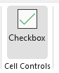
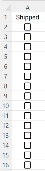
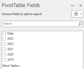
In Excel’s latest version, a checkbox can be added right from the Insert tab on the ribbon. Simply clicking on the checkbox button will insert a checkbox into your spreadsheet. To insert multiple checkboxes at once, first select all the cells which you want to contain checkboxes. Then, click on the checkbox button. The cells will now be filled with checkboxes.

Using checkbox selections in formulas

If a checkbox is selected, its value becomes TRUE, and FALSE if it is unchecked. Using an IF function, I can create a formula to check whether the value is TRUE or not, and based on that, determine the output. In the following example, I use checkboxes to determine if something has been received. If it is checked off, then the value is “Received” and if it’s not, then it will say “Not Received”

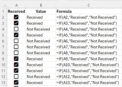
Excel spreadsheet using checkboxes to determine if something was received or not.

The formula is a straightforward and can be used to track whether something has been processed or not.

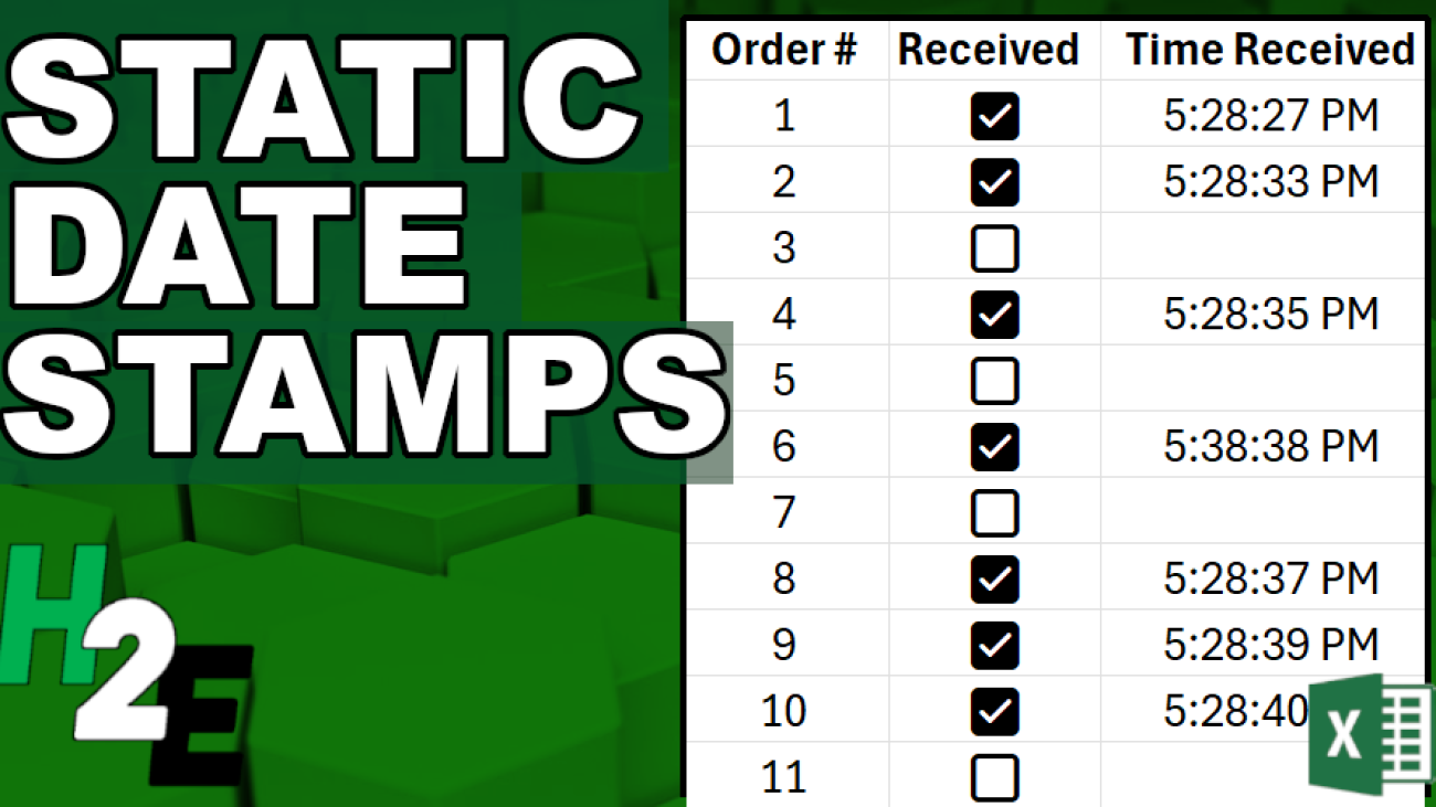
Creating a static timestamp in Excel using a checkbox

Let’s use a more complex situation in Excel, such as when we want to lock in the time of when someone received the order, not simply whether or not they received it. This involves a bit more complexity and we’ll need to allow for some circular references in this case, which is usually a no-no in Excel.

Here’s how we can get this scenario to work. Assuming the checkboxes are still in column A, the formula for cell B2 would be as follows:

=IF(A2,IF(B2=””,NOW(),B2),””)

The first argument in the IF statement checks to see if the checkbox is selected. It looks at A2 to see if it returns a value of TRUE or FALSE. Since it is a boolean argument, it is not necessary to state A2=TRUE; that goes without saying in this example.

If that condition is met, we move on to the next IF function. This one checks if B2 (the current cell, and thus, creating a circular reference) is blank. If it is, then the current date and time would be inserted with the NOW function. If it isn’t blank, then the value in B2 would remain as it is. And if the checkbox is A2 isn’t checked off at all, the value in B2 will be blank.

This formula initially won’t work and will give you an error stating that you’ve created a circular reference. To fix this, you need to allow for Iterative Calculations. This will ensure that Excel stops calculating after a certain number of attempts and take the last value. To activate this, go into Excel Options and under Formulas, select to Enable iterative calculation:

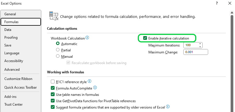
Enabling iterative calculations in Excel.

You can leave the default number of iterations. Now, your formula will calculate without the circular reference error. And when you check off boxes, the timestamps will all remain static until the checkboxes become unchecked again.

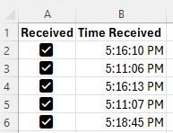
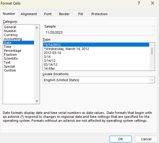
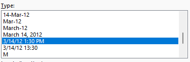
Checkboxes in Excel showing the time received.

In the above screenshot I only show time, but that’s because I have formatted it to only show time. Since the NOW function contains both date and time, you can choose to show both, or just time or date individually.

The drawbacks of iterative calculations

Before you enable iterative calculations, however, you should consider the risks with doing so:

Performance Issues. Iterative calculations can significantly slow down Excel, especially in large and complex worksheets. Excel has to repeatedly recalculate formulas until either the maximum number of iterations is reached or the difference between the results of two calculations is below a certain threshold. This can be particularly noticeable if the workbook contains many formulas or data points.

Accuracy and Precision. The result of an iterative calculation can depend on the maximum number of iterations and the maximum change settings. If these are not appropriately set, the result may be inaccurate or not precise enough for your needs. This is because the calculation stops once the set limits are reached, not necessarily when the correct or most accurate result is found.

Risk of Other Circular Reference Errors. While iterative calculations allow you to use circular references intentionally, they also increase the risk of unintended circular references. Unintended circular references can lead to errors and incorrect data, making it difficult to debug and correct issues within your workbook.

Compatibility Issues. If you share your Excel workbook with users who have iterative calculations disabled, or if the workbook is opened in a different spreadsheet program that doesn’t support iterative calculations, the intended functionality may not work correctly. This can lead to errors or data inconsistency.

Potential for Infinite Loops. Incorrectly configured iterative calculations can lead to infinite loops, where Excel continuously recalculates without reaching a conclusion. This can cause Excel to freeze or crash, potentially leading to data loss if changes haven’t been saved.

As long as you understand the risks of enabling iterative calculations, they can help you in setting static date and time stamps in Excel.

If you like this post on Adding Static Timestamps in Excel Using Checkboxes please give this site a like on Facebook and also be sure to check out some of the many templates that we have available for download. You can also follow me on Twitter and YouTube. Also, please consider buying me a coffee if you find my website helpful and would like to support it.

Create a Date and Time Stamp in Excel Using VBA

November 28, 2023

by howtoexcel dates functions vba

Do you have a spreadsheet that needs to track dates? Whether it’s a shipping log, an inventory tracker, a sales order template, or just something to track when the last change was made to a cell, there’s an easy way you can create a date stamp in Excel with VBA.

Use checkboxes to make your spreadsheet more user friendly

If you have a spreadsheet where you want to track statuses, using checkboxes can be helpful. This way, someone can check or uncheck the status of an order. This can indicate whether it has been shipped, ordered, or completed. Excel has made it easier to insert checkboxes with a recent update. If you’re using Microsoft 365, then on the Insert tab on the Ribbon, you should see an option to insert a Checkbox:

Selecting to insert a checkbox into Excel.

When you click on this button, it will insert a checkbox right into the active cell that you’re on. Want to insert checkboxes into multiple cells at once? Simply select a range of cell and then click on the button:

If a checkbox is checked, its value is TRUE. If it is unchecked, then the value is FALSE. This is important to know when creating formulas.

Populating the date using the NOW() function isn’t useful for date stamps

If you want to enter the current date into a cell, you can use the CTRL+; shortcut. The problem is that it won’t change if you go to uncheck and re-check a checkbox. It’s a stale value and it isn’t a formula.

What you may be tempted to use is the NOW() function. However, the limitation here is that anytime the cell recalculates, it will refresh with the current date and time. It won’t hold the existing date stamp. You can create a circular reference and adjust iterative calculations. But there’s an easier way you can create a date stamp in Excel with just a few lines of code using VBA.

Creating a custom function using VBA

You can create a custom function with VBA. To do, start by opening up your VBA editor using ALT+F11. On the Insert menu, select the option for Module. There, you’ll have an empty canvas to enter code on. The custom function can simply contain one argument — the cell that contains the checkbox. This is to determine whether it is checked (TRUE) or unchecked (FALSE). If it is checked, then the timestamp will be equal to the current date and time. If it’s unchecked, then the timestamp will be blank, and so will the cell value.

Here’s the full code for the function:


Function timestamp(checkbox As Boolean)

    If checkbox = True Then
        
        timestamp = Now()
    
    Else
    
        timestamp = ""
    
    End If
    

End Function

This function is now created. To use it within your spreadsheet, all you need to do is select a cell where you want the date and time to populate on. Then, assuming your checkbox is in cell A2, enter the following formula:

=timestamp(A2)

This will run through the VBA code to determine whether to populate the current date and time or not. Since there is no NOW() function present in this formula, it won’t recalculate with the current date.

Formatting your date and time

Even if the custom function work, you may notice that the value that it populates doesn’t look right. If you get a number or the time is missing from the date, then you’ll need to modify the cell format. To do that, select the cell and press CTRL+1. Then, select the Date category where you’ll see various date formats:

If you scroll down the list, there will be an option that shows the date and time:

If you use that format, then your date will now look correct, including both the date and time.

If you like this post on How to Create a Date and Time Stamp in Excel Using VBA, please give this site a like on Facebook and also be sure to check out some of the many templates that we have available for download. You can also follow me on Twitter and YouTube. Also, please consider buying me a coffee if you find my website helpful and would like to support it.

How to Group Dates by Month in a Pivot Table

August 8, 2023

by howtoexcel analysis dates financial analysis pivot table

In this post, I’m going to show you how to group dates in a pivot table by month. By doing this, you can do analysis by month rather than individual day. And that will also make it easier to plot the data on a chart.

For this example, I’m going to use TSA passenger volumes as my data set and analyze them by month and year. Here is the data I’m going to use, which runs up until Aug. 6, 2023:

If I load this into a pivot table, my fields are as follows:

Pivot table fields for TSA passenger volume data.

I have the date field which shows the current year’s dates. And there is also a field for each year, which contains the passenger volumes. If I put the Date in the Rows section of the pivot table and then years into the values section, then my pivot table looks like this:

Pivot table summarizing TSA traffic volumes by year.

There are a few things that I need to fix for this analysis to work:

I need to change each year field so that it is taking an average instead of summing the values. If I leave it as is, summing the values may not be helpful as the months are not going to be identical eah year. Taking an average will help smooth the data.
The formatting should be changed so that the values are separated by commas. This will make it easier to visually see the data. The numbers are too big and can be difficult to interpret in their current format.
The Row labels are broken down by year. But I already have the year values going across. This is not necessary and I need to have only the month values.

Here’s how to address these items.

To change the year field so that it takes an average, right-click on the field and select the option to summarize as an average:

Changing how to summarize values by in a pivot table.

Repeat this for each field, so that everything says average. To fix the number formatting, right-click on each field and select Value Field Settings:

Changing the value field settings in a pivot table.

Change the formatting to Number and check off the option for the 1000 separator. Repeat these steps for the other fields as well.

Next, for the date grouping, right-click on any of the date values and select the Group button:

At the following dialog box, uncheck years and quarters and just leave Months:

Grouping dates by month only in a pivot table.

After making all those changes, my pivot table now looks like this:

A pivot table summarizing passenger volumes by year and month.

It’s now easier to compare the different months and years. And it’s also easier to put it on a chart. If I insert a line chart, it’s easy to spot the trends by a monthly and yearly basis:

A chart comparing passenger volumes by year and month.

This is a PivotChart, as it evident from the grey drop-down options. If you prefer to get rid of the filters, go to the PivotChart Analyze tab and uncheck the Field Buttons option. Now you’ll have a cleaner chart layout. In the below example, I have also moved the legend to the bottom:

Chart showing passenger volumes by month and year.

As you can see, by grouping your pivot table dates by month, it becomes easier to analyze data. And by not doing a daily analysis, it’s possible to look at the data from a year-to-date view to compare the monthly averages. This way, you are able to still see the story behind the data without having a crowded chart.

If you liked this post on How to Group Dates by Month in a Pivot Table, please give this site a like on Facebook and also be sure to check out some of the many templates that we have available for download. You can also follow me on Twitter and YouTube. Also, please consider buying me a coffee if you find my website helpful and would like to support it.

15 Excel Functions Accountants Should Know

March 28, 2023

by howtoexcel accounting advanced average averages beginner count countif dates functions index intermediate lookup lookups match sum sumif sumifs unique vlookup

If you’re an accountant, you know that working with large amounts of data can be a daunting task. But with Excel, that work can get a whole lot easier and more efficient. Understanding Excel’s advanced features and functions can improve productivity, reduce errors, make your work more accurate, and most importantly — save you time. Below, I’ll go over some of the most important Excel functions that accountants should know, and provide examples of how to use them. For this example, I’ll use the following spreadsheet. Feel free to download it and follow along with the calculations.

1. SUM

The SUM function is a basic but essential function in Excel. It allows you to add up a range of values, which is helpful when calculating totals, such as revenue, expenses, and profits. Suppose you have a spreadsheet with sales data. In the above example, the total sales are in column G. If you wanted to sum up the entire column, the formula would be as follows: =SUM(G:G)

2. AVERAGE

The AVERAGE function calculates the average of a range of values. It is useful when analyzing data and preparing financial statements. In the above example, suppose you wanted to calculate what the average sale was. To do this, you can just use the AVERAGE function on column G, similar to the SUM function before. Here’s the formula: =AVERAGE(G:G)

3. IF

The IF function allows you to test a condition and return one value if the condition is true and another value if the condition is false. This can be useful because it can send your formulas to the next level. By knowing to use the IF function, you could also use SUMIF, AVERAGEIF, and many other functions that involve an if statement. In the above example, let’s say you only wanted to know if a value in cell M2 was part of the Motorcycles product line. The formula would be as follows: =IF(M2=”Motorcycles”,1,2). If it is part of Motorcycles, you would have a value of 1, otherwise, it would be 2.

4. SUMIF

By knowing the SUM and IF functions, you can combine them together with SUMIF, which is an incredibly popular function. It gives you a quick way to tally up the totals that meet a criteria. For example, let’s say you want all sales that relate to the Motorcycles category. The formula for that would be as follows: =SUMIF(M:M,”Motorcycles”,G:G). If the criteria is met in column M, then the formula will sum up the corresponding values in column G. There’s also the super-powered SUMIFS function, which allows you to combine multiple criteria.

5. EOMONTH

The EOMONTH function calculates the last day of the month for a specified number of months in the future or past. It is useful when working with data that is organized by date. For accountants, this can be useful when you’re calculating when something is due. Let’s say in this example, we need to calculate the date orders need to go out on, and that needs to be the end of the next month. Using the ORDERDATE field in column H, here’s how that calculation would look in the first cell, which would then be copied down for the rest: =EOMONTH(H2,1)

6. TODAY

The TODAY function is helpful for accountants in calculating deadlines and knowing how many days are remaining or past a certain date. Suppose that you wanted to know how many days have past since the ORDER DUE DATE that was calculated in the previous example. Rather than entering in a static date that every day you would need to change, you can just use the TODAY function. Here’s how a formula calculating the days since the deadline for the first cell would look like, assuming the due date is in column N: =TODAY()-N2. The next day you open up the workbook, the calculations will update to reflect the current date; there’s no need to make any changes. There are many more date calculations you can do in Excel.

7. FV

The FV function calculates the future value of an investment based on a fixed interest rate and a regular payment schedule. You can use it to calculate the future value of an investment or savings account. Let’s say that you wanted to save $10,000 per year and expect to earn a return of 5% per year on that investment. Using the FV calculation, you can do that with the following formula: =FV(0.05,5,-10000). If you don’t enter a negative for the payment amount, the formula will result in a negative value. You can also specify whether payments happen at the beginning of a period (1) or end (0 — this is the default) with the last argument in the function.

8. PV

The PV function lets you do the opposite and work backwards from a future value to the present. Knowing that the calculation in example 7 returns a value of $55,256.31, that can be used in the PV calculation to check our work: =PV(0.05,5,10000,-55256.31). The formula returns a value of 0, which is correct, as there was no starting value in the FV calculation.

9. PMT

The PMT function calculates the periodic payment required to pay off a loan with a fixed interest rate over a specified period. It is helpful when determining the monthly payments required to pay off a loan or mortgage. Let’s take the example of a mortgage payment where you need to pay down $500,000 over the period of 30 years, in monthly payments. At a 5% interest rate, here’s what the payment calculation would be: =PMT(0.05/12,12*30,-500000,0). Here again the ending value needs to be a negative to avoid a negative value in the result. And since the payments are monthly, the periods need to be multiplied by 12 and the interest rate is dividend by 12.

10. VLOOKUP

The VLOOKUP function allows you to search for a value in a table and return a corresponding value from another column in the same row. It’s one of the most common Excel functions because of how useful and easy to use it is. It is helpful when working with large data sets and performing data analysis. Let’s suppose in this example that you want to find the sales related to order number 10318. The formula for that calculation might look like this: =VLOOKUP(10318,C:G,5,FALSE). In a VLOOKUP function, you need to specify the column number you want to extract from, which is what the 5 represents. If you’re using Office 365, you can also use the newer, flashier XLOOKUP function. I put VLOOKUP on this list because it’ll work on older versions of Excel — XLOOKUP won’t.

11. INDEX

The INDEX function allows you to return a value from a data set by specifying the row and column number. It’s also helpful if you just want to return data from a single row or column. For example, the sales column is in column G. If I know the order number is on row 20 (which relates to order number 10318), this formula would do the same job as the VLOOKUP in the previous example: =INDEX(G:G,20,1).

12. MATCH

The MATCH function allows you to find the position of a value within a range of cells. Oftentimes, Excel users deploy a combination of INDEX and MATCH instead of VLOOKUP due to its limitation (e.g. VLOOKUP can’t extract values to the left of the lookup field). In the previous example, you had to specify the row belonging to the order number. But if you didn’t know it, you could use the MATCH function within the INDEX function. The MATCH function would look like this: =MATCH(10318,C:C,0). Placed within an INDEX function, it can replace the argument where in the previous example, we set a value of 20: =INDEX(G:G,MATCH(10318,C:C,0),1). By doing this, you have a more flexible version of the VLOOKUP function. You can also create dynamic formulas using INDEX and MATCH that use lookups for both the column and row.

13. COUNTIF

The COUNTIF function allows you to count the number of cells in a range that meet a specified condition. Let’s count the number of values in the data set that are Motorcycles. To do this, you would enter the following formula: =COUNTIF(M:M,”Motorcycles”).

14. COUNTA

The COUNTA function is similar to the previous function, except it only counts the number of non-empty cells. With no criteria, it is helpful to just the total number of values within a range. To calculate how many cells are in this data set, you can use the following formula: =COUNTA(C:C). If there are no gaps in data, then the result should be the same regardless of which column is used. And when combined with the UNIQUE function, you can have an easy way to count the number of unique values.

15. UNIQUE

The UNIQUE function returns a list of unique values within a range, and it’s a much easier method than the old-school way of extracting unique values. If you wanted to extract all the unique product lines in column M, you would enter the following formula: =UNIQUE(M:M). If, however, you just wanted to count the number of unique values, you could embed it within the COUNTA function as follows: =COUNTA(UNIQUE(M:M)). You can adjust your range if you don’t want to include the header.

This is just a sample of some of the useful Excel functions that accountants can utilize. If you are familiar with them, you’ll put yourself in a great position to improve the efficiency of your workflow and make your spreadsheets easier to use. Plus, you can confidently say that you are highly competent with Excel, which can make your resume more attractive and make you better suited for accounting jobs that require advanced Excel skills — and there are many of them that do!.

If you liked this post on 15 Excel Functions Accountants Should Know, please give this site a like on Facebook and also be sure to check out some of the many templates that we have available for download. You can also follow me on Twitter and YouTube. Also, please consider buying me a coffee if you find my website helpful and would like to support it.

How to Convert Date Formats in Excel

March 21, 2023

by howtoexcel dates

If you’ve ever downloaded data and received dates in the wrong format, it can be a challenge to fix. If your regional settings are month/day/year but in a spreadsheet they are in day/month/year format, then odds are they will be reading in a text format rather than date. The one exception is when you’re dealing with month and day values that are 12 or less, and thus, they could be both month or day values. In those cases, the values are still reading as dates, but they are still incorrect. Here’s how you can fix all of these issues by using a formula.

Converting text date formats using TEXTSPLIT and INDEX

Suppose you have the following values, which are for March 2023:

Date values that are in the wrong format in an Excel spreadsheet.

These dates are not in the month/day/year format. However, only the value that has a 13 at the start is aligned to the left — indicating that it’s a text value. The others are recognized as dates, even though they are in the wrong format. This is what can make this calculation tricky, to accommodate both situations — but it’s not impossible.

First, let’s deal with the values that are in text. For these ones, their values just need to be parsed out. In the past, you could do this with a complicated series of LEN, MID, LEFT, and RIGHT functions. However, thanks to the relatively new TEXSPLIT function, it’s easier to do that.

Here’s how you would parse out the data if it’s in a text format, such as in the last instance (March 13), which is in cell A14:

=TEXTSPLIT(A14,”/”)

This formula will break out the data into an array:

This isn’t the final solution, as this would still require another formula to pull these values into a date. And to accomplish that, this is where the INDEX function comes into play. Since there are three values here, using INDEX, you can select which value goes in which argument for the DATE function.

For instance, the following formula would extract the first value before the /, which is the number 13:

=INDEX(TEXTSPLIT(A14,”/”),1,1)

For the second number, 3, the column argument needs to change to a 2, to get the second column in the array:

=INDEX(TEXTSPLIT(A14,”/”),1,2)

And for the last one, the column would be set to 3:

=INDEX(TEXTSPLIT(A14,”/”),1,3)

Together, these values can be put within a DATE function. The arguments in the DATE format are in the following order: year, month, day. That means that last value in the array (position 3) needs to be first, followed by the second position (the month), and the last position (for the day). Here’s how that formula looks:

=DATE(INDEX(TEXTSPLIT(A14,”/”),1,3),INDEX(TEXTSPLIT(A14,”/”),1,2),INDEX(TEXTSPLIT(A14,”/”),1,1))

It’s the same formula repeated but referencing different column positions. And now, the formula gives me the date in the correct month/day/year format:

However, this formula won’t work on the other values; they will result in errors since those are date values and only display slashes but don’t actually contain them the way a text value does. However, the solution for these formulas is even easier.

How to rearrange date values

Since the below cells read as date values, we can reference their respective month, day, and year values, and simply put them back into the DATE function.

Date values in Excel that are in day/month/year format.

The first value is the day value, followed by the month, and then the year. However, my regional settings are set to month/day/year format. That means if these cells are reading as date values, which they are, then that means the first value is going to be the month. By using the MONTH function, I can get that first value. But the key is, when I’m creating a new formula and using the DATE function, I will need to put that value in the argument that relates to the day. This can be a bit tricky and remember, if your regional settings are different from mine, you will need to alter your formula to ensure the right value is going into the right argument.

Similarly, for the second value (which corresponds to the day in my regional settings), I will use the DAY function to get that value. But I will actually put it in the month argument.

Lastly, the YEAR function will extract the year and go into the same year argument position, since month/day/year and day/month/year have the same position for the year. Here’s how this formula looks in its entirety, grabbing all the different values:

=DATE(YEAR(A2),DAY(A2),MONTH(A2))

By copying the formulas, the date formats now look correct:

Converting day/month/year dates into month/day/year.

Combining the formulas

There’s just one left piece left in all of this, and that’s combining the two formulas so they can accommodate both situations: when the data is in text format, and when it’s reading as a date. This can be done by using the ISTEXT function, to check if a value is reading as text or not. If it’s a text value, then it will use the TEXTSPLIT function. Otherwise, it will simply reposition the date values. Here’s the formula that will factor in both situations:

=IF(ISTEXT(A2),DATE(INDEX(TEXTSPLIT(A2,”/”),1,3),INDEX(TEXTSPLIT(A2,”/”),1,2),INDEX(TEXTSPLIT(A2,”/”),1,1)),DATE(YEAR(A2),DAY(A2),MONTH(A2)))

Now, this one formula can be used on all of the cells, whether they are in date or text format.

If you liked this post on How to Convert Date Formats in Excel, please give this site a like on Facebook and also be sure to check out some of the many templates that we have available for download. You can also follow me on Twitter and YouTube. Also, please consider buying me a coffee if you find my website helpful and would like to support it.

How to Show Elapsed Time in Excel

January 10, 2023

by howtoexcel dates formatting

Do you need to calculate the time that that has elapsed between two date values in Excel? In this post, I’ll show you how you can show the difference in hours, minutes, and seconds. This can be useful if you need to determine hours on a work shift or just to see how much time is remaining until a deadline.

The following table is what an employee’s shift schedule might look like over the course of a week:

You have the time they started work, left work, and the duration of their break. To calculate the time difference and net hours worked, this can be accomplished by the following formula:

Time Work : Time Out – Time In – Break

It’s just a simple subtraction formula. However, the tricky part is that by default, Excel will calculate this difference in days and so the result will be shown as a fraction of a day (since it is less than 24 hours):

Total shift hours in Excel shows as a fraction of a day.

There are a couple of ways to fix this. The first way is to multiply the results by a factor of 24 so that the calculation gets converted into hours:

Total shift hours in Excel when taking fractions of a day and multiplying them by 24.

The caveat here is that now instead of fractions of a day, you now have fractions of an hour. If you prefer to not do any conversions and instead just want to display the value as elapsed time as hours and minutes, that can be done by formatting the cells, which is the alternative method.

To do this, select the cells in the Total Time column and select CTRL+1 to Format Cells. From there, go to the Custom category and enter [h]:mm as follows:

Modifying the number format to show elapsed time in Excel by using the [h]:mm format.

By doing this, the result will be similar to when you multiplied the values by 24:

An important difference you’ll notice is that the Total Time column shows in terms of hours and minutes, whereas the Hours column still shows fractions of an hour. For instance: 9 hours and 30 minutes shows up as 9:30 in Total Time but under the Hours column it is 9.50. One column is showing the actual minutes while the other is showing it in terms of fractions of an hour.

If you wanted to only show the number of minutes elapsed, the time format would simply be [m]. Then, your time would show in terms of minutes.

Showing elapsed time in terms of minutes in Excel by using the [m] format.

And to show the time in seconds, use [s]:

Showing elapsed time in Excel in terms of seconds using the [s] format.

You could, of course, do all of these conversions by multiplying the hours field by 60 to convert it into minutes and then by 60 again to convert into seconds. By just changing the number format, you aren’t doing any changes to the original calculation. Either option can get the desired end results. However, if you want to specifically show hours and minutes and seconds, and not fractions of an hour, you’ll want to use either [h]:mm or perhaps [h]:mm:ss if you have your time broken down to the second.

If you liked this post on How to Show Elapsed Time in Excel, please give this site a like on Facebook and also be sure to check out some of the many templates that we have available for download. You can also follow us on Twitter and YouTube.

How to Calculate Age in Excel

September 27, 2022

by howtoexcel with No Comment dates functions

Excel’s date and time functions make it easy to calculate the difference between two dates. And in this post, I’ll show you how you can calculate age in Excel. This can include a person’s age, or the interval between two dates. You can also break this difference into years, months, days, minutes, and seconds.

Use the YEARFRAC function to calculate the time in terms of fractions of years

One of the easiest ways to calculate age is by using the YEARFRAC function. As the name suggests, it will give you the fraction of a year. Suppose you wanted to calculate the difference between the start of the year 2000 and Christmas 2022. This is what your formula would look like:

=YEARFRAC("1/1/2000","12/25/2022")

Note that depending on your regional settings, you may need to enter date values in different formats. Alternatively, you could simply reference cells that contain date values so that you don’t need to do any hardcoding here.

The above formula will return a value of 22.983. Since Christmas falls towards near the end of the year, the number is close to 23. If instead you choose Jan. 31, 2022 as the end date, then the formula would return a value of 22.083.

Use the TODAY function to make your formula dynamic

To calculate age so that it is always going to be up until today’s date, you can use the TODAY function. This avoids you having to enter the current date each time you want an up-to-date calculation. For example, if you wanted to calculate the fractional years between the start of 2000 and today, your formula would look like this:

=YEARFRAC("1/1/2000",TODAY())

The TODAY value will automatically update so you don’t need to do anything to trigger that calculation. Just by opening your workbook, Excel will pull in the current date value, and your formulas that contain the TODAY function will adjust accordingly.

Calculating month, day, hour differences

If you want to calculate the difference in months rather than fractions of years, there’s an easy way you can do that as well. Excel has a DATEDIF function that can make that process quick and easy. The logic is the same as with the earlier formula, but the main difference is that you enter “m” for a third argument, indicating month. Here’s the formula, using the same values as earlier:

=DATEDIF("1/1/2000","1/31/2022","m")

This formula gives a result of 264, which equates to 22 years. You’ll notice the drawback here is there are no fractions or rounding, just 264 months. If I adjust the end date to the start of February (“2/1/2022”), then it will return a value of 265 months. Until the month is complete, the formula won’t add the extra month, even if you’re selecting a date that’s nearly at the end (e.g. January 31).

One alternative you can make is to calculate the difference in days:

=DATEDIF("1/1/2000","1/31/2022","d")

This formula will return a value of 8,066. If you were to divide this by 365, you would get 22.09863. That’s the same answer I would get using the YEARFRAC function if I entered the last (optional) argument in that function to specify that I wanted to use 365 days for my calculation (the default calculation uses 360).

DATEDIF doesn’t have an argument that lets you calculate hours or minutes. However, with the number of days, you can approximate that by multiplying by hours. If you did want to get to that precise level of detail, you would need to create a separate formula for hours and minutes — and you would also need to ensure your date values included that level of detail to avoid approximation.

Using the HOUR, MINUTE, and SECOND functions, you can subtract the starting date from the ending date to arrive at a difference for each of those time calculations.. For these types of details, you should reference the cells as opposed to key in the hour, minute, and second values to ensure everything is entered correctly.

Calculating date differences using the days, month, minutes, seconds, and yearfrac functions.

If you liked this post on How to Calculate Age in Excel, please give this site a like on Facebook and also be sure to check out some of the many templates that we have available for download. You can also follow us on Twitter and YouTube.

Excel’s New Text Functions Make Data Parsing a Breeze

April 13, 2022

by howtoexcel with No Comment dates functions parse

Parsing data in Excel can be complicated, using a combination of functions ranging from LEFT, RIGHT, MID, and FIND. However, with the help of a few new functions that are available in Excel, the process is a whole lot easier for users. In this post, I’ll look at how you could parse out a date that is formatted as text using the new functions and comparing that with how you might have done it using the old functions.

In this example, I’m going to try parse out the numbers I need to convert the following value, which is reading as text:

This date is April 19, 2022. But because my regional settings are set to month/day/year this value doesn’t compute properly since it would be looking for a 19th month.

Pulling the day value (data before the delimiter)

The old method

The first number in the date value above relates to the day of the month. Using the LEFT function in Excel, you could use something like this:

=LEFT(X,2)

Where X is the cell value. That will pull the first two characters in the string. But in some cases there might only be one day for the date. And for that reason, I’m not going to hardcode the number of characters. The best approach (under the old method) is by using the FIND function to locate where the delimiter (“/”) is. The more versatile formula would look as follows:

=LEFT(X,FIND("/",X,1)-1)

The new method

One of Excel’s new text functions is called TEXTBEFORE. And as the name suggests, it will extract all the text that comes before a delimiter. Without needing the FIND function, I can simply do this to extract the day value:

 =TEXTBEFORE(X,"/")

Pulling the year value (data after the delimiter)

The old method

To grab the year in the date I could cheat and use the RIGHT function and just grab the last four numbers. But that wouldn’t be flexible enough in the event that I might have 2 digits instead of 4 as the year. This can get messy as now I have to use multiple FIND functions in order to determine the length. The key is to take the length of the function and subtract from that the position of the second delimiter. Here’s what that looks like:

=RIGHT(X,LEN(X)-FIND("/",X,FIND("/",X,1)+1))

The nested FIND functions can get a bit complicated. Here you’ll see even more efficiency with Excel’s new functions.

The new method

The TEXTAFTER function can greatly simplify this action because you can specify after which delimiter you want to pull the characters; there is no need to have nested functions with this:

=TEXTAFTER(X,"/",2)

In this formula, the characters after the second “/” will be extracted. Note: both the TEXTBEFORE and TEXTAFTER functions allow you to specify the instance of the delimiter (i.e. it doesn’t always need to be the first one).

Pulling the month value (data between delimiters)

The old method

The most challenging part of this process is undoubtedly to pull the data between delimiters. In this example, I’ll need to use the MID function and use nested FIND functions to determine the space in-between the delimiters. It’s an ugly formula if you don’t rely on hardcoding:

=MID(X,FIND("/",X,1)+1,FIND("/",X,FIND("/",X,1)+1)-FIND("/",X,1)-1)

That’s four FIND functions in one formula. You can quickly see how parsing out this information can be a challenge. But with the new Excel functions, it’s much easier to do this.

The new method

There isn’t a new function that specifically pulls the values between delimiters. But by using both the TEXTAFTER and TEXTBEFORE functions, you can do exactly that. Let’s start with just grabbing everything after the first delimiter:

TEXTAFTER(X,"/")

This will give us the following result: 4/2022. Obviously that’s not what I want. But now, I can nest this within the TEXTBEFORE function, and grab the value before that other “/” with the following formula:

=TEXTBEFORE(TEXTAFTER(X,"/"),"/")

We are still dealing with a nested function here, but this is no doubt easier than all those FIND functions under the old method.

Using an array function

Another option that you can use is to extract all the values between the delimiters using the TEXTSPLIT function. Simply enter the following formula:

=TEXTSPLIT(X,"/")

Then the values will be extracted into three cells, one for the day, month, and year:

The benefit of this approach is you can quickly pull everything from the cell you’re parsing data from.

Regardless of which option you choose, Excel has given its users some new tools that can make the parsing much easier and less complicated than it was before.

If you liked this post on Excel’s New Text Functions, please give this site a like on Facebook and also be sure to check out some of the many templates that we have available for download. You can also follow us on Twitter and YouTube.

Calculate the First Day and Last Day of the Week

January 26, 2022

by howtoexcel with No Comment calendar dates

Excel’s WEEKNUM function can return the specific week that a date falls in. But to do the reverse is a bit more challenging. In this post, I’ll show you how you can get the first and last day of a week (as well as anything in-between).

Setting up some variables

You can make this into a large and complex formula, but I’m going to make it a bit more organized by utilizing named ranges. The two names ranges I’m going to set up are for the day of the week (DAYNUMBER) that I want to calculate for, and the first day of the year (FIRSTDAY).

I’m going to use Monday as the day of the week my week starts on. On my regional settings, that is weekday #2. If you’re not sure about yours, you can use the WEEKDAY function on a day that is a Monday (or whichever day you wish to use) to determine the number associated with that.

Calculating the difference between the first day and your desired day of the week

The day the year begins on serves as an important starting point. This year began on a Saturday. If my desired day is Monday, then I need to calculate the difference between those days of the week. The formula for that would be as follows:

=DAYNUMBER - WEEKDAY(FIRSTDAY)

This returns a value of -5. If I wanted to know when the first Monday of the year was, I couldn’t just deduct 5 from the first day or I’d end up in the wrong year. What I need to do is to set up an IF function to say that if the difference is negative, I will add 7 to adjust for that fact. And if it isn’t negative, then I can just add to the starting date. Here is my formula thus far:

=IF(DAYNUMBER-WEEKDAY(FIRSTDAY)<0,DAYNUMBER-WEEKDAY(FIRSTDAY)+7,DAYNUMBER-WEEKDAY(FIRSTDAY))

To get to the right day, I need to add this to my starting date:

=FIRSTDAY+IF(DAYNUMBER-WEEKDAY(FIRSTDAY)<0,DAYNUMBER-WEEKDAY(FIRSTDAY)+7,DAYNUMBER-WEEKDAY(FIRSTDAY))

Using the above formula, Excel tells me that Jan. 3, 2022, was the first Monday of the year, which is correct. But I need to adjust the formula to ensure the calculation puts me in the correct week.

Adjusting for the week number

The above formula works if I want the first week. If I want it to be more flexible than that, I need to include the week number in my calculation. For that, I’m going to create a named range called WEEK. The key is in adjusting the +7 calculation. In the first argument of my formula, when it was negative, I added 7. If I want the second week, then I need to add it by another factor of 7. Here’s how that part of the formula would look:

WEEK-WEEKDAY(FIRSTDAY)+(7*WEEK)

I also need to add that part to the second argument, which currently doesn’t adjust for the week number:

WEEKDAY(FIRSTDAY)+(7*(WEEK-1))

The completed formula is as follows:

=FIRSTDAY+IF(DAYNUMBER-WEEKDAY(FIRSTDAY)<0,DAYNUMBER-WEEKDAY(FIRSTDAY)+(7*WEEK),DAYNUMBER-WEEKDAY(FIRSTDAY)+(7*(WEEK-1)))

Now I can adjust the calculation for different days of the week and different week numbers. And so whether you’re looking at the first day of the week or the last day of the week, you can just adjust the day number you’re looking for.

Here’s what the formula would look like without named ranges if the year was the current year and it was pulling the Monday of the 50th week of the year:

=(DATE(YEAR(NOW()),1,1)+IF(2-WEEKDAY(DATE(YEAR(NOW()),1,1))<0,2-WEEKDAY(DATE(YEAR(NOW()),1,1))+(7*50),2-WEEKDAY(DATE(YEAR(NOW()),1,1))+(7*(50-1))))

If you liked this post on How to Calculate the First Day and Last Day of the Week, please give this site a like on Facebook and also be sure to check out some of the many templates that we have available for download. You can also follow us on Twitter and YouTube.

How to Convert Month Number to Month Name in Excel

June 21, 2021

by howtoexcel with No Comment beginner calendar dates formatting tips & tricks

Do you have a report in Excel that lists the months as the numbers 1 through 12 and you want to convert that into the actual month names? Below, I’ll show you how you convert a month number into a month name in Excel.

Here’s an example of data that shows monthly sales but it only lists the number as opposed to the name:

Sales by month with the month number showing in digits.

If you had the entire date in a cell you could format it so that it showed the month. For instance, what I could do is type in =TEXT(A1,”MMM”) which would convert the value in cell A1 into a three-letter abbreviation for the month. But the numbers 1 through 12 will return values of “Jan” as Excel will think that you are referring to the first month of the year.

However, that changes once you get to the number 32. Since there are only 31 days in January, the number 32 will return a value of “Feb” if you were to continue on with that formula. And so the trick is to multiply these values all by a factor of 28. Since that’s the minimum number of days every month will have, it ensures that jumping by 28 each time will put you into each month of the year. This is what my values will look like:

To prove this out, here is which dates those days of the year would correspond to:

Day of the year along with the corresponding date.

In month 12, we barely make it in December using this approach but that’s good enough. And even in a leap year, multiplying by 28 still works. In this example, I include 2024, the next year that February gets an extra day:

Day of the year along with the corresponding date, including a leap year.

So now that we’ve confirmed that those numbers will fall within the correct months, we can use the TEXT formula noted above to convert those numbers into month dates, and this is what we end up with:

Month numbers converted into month names.

You can also multiply by 29 and this logic will still work. But if you use 27 then your months will be wrong by the time you hit September and if you use a multiple of 30, then in non-leap years you will be jumping too quickly and you will have two dates in March.

If you liked this post on How to Convert Month Number to Month Name in Excel, please give this site a like on Facebook and also be sure to check out some of the many templates that we have available for download. You can also follow us on Twitter and YouTube.