IF Functions: Calculating Data If Criteria Is Met

 =IF(A1=”A”,1,0)

In this example, if A1 is equal to the letter A then the result of the formula is 1. If it is equal to B, C, or anything else, the result will be 0. It will look for an exact match – if you don’t want an exact match, you’ll need to use wildcards (see later down).

You can make nested If functions as well – instead of putting  a 0 in the formula above you can add another if function:

=IF(A1=”A”,1,IF(A1=”B”,2,0))

In this formula, if the cell A1 does not match A, then it will do another test. The second test is checking to see if it matches B – if it does, it will assign a value of 2, and if not, a value of 0. You can keep adding If functions as much as you need to. But keep track of the parentheses to make sure they are properly closed. If you find yourself having to do many nested if functions then you may be better off using a lookup formula.

The COUNTIF formula counts the number of items your criteria is met. See the example below:

Example 3

=COUNTIF(A1:A7,”A”)

This formula is looking at all the cells in the range A1:A7 and counting them if the match the letter A. This would result in 5. 

In newer versions of Excel, there is a plural version of COUNTIF– COUNTIFS. This allows you to use multiple criteria:

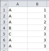
=COUNTIFS(A1:A7,”A”,B1:B7,1)

This formula builds on the last, where it looks for the value A in cells A1:A7 and then also looks for the number 1 in cells B1:B7. This would result in 2. As there are two instances where A and 1 are in the same row. 

Note: If your ranges are not identical (e.g. A1:A7 and B1:B6), your formula will not work properly. Also, because in this example the formula was looking for a number, it does not have to be in quotations. You can keep adding more criteria by adding another comma instead of closing the formula.

SUMIF function works similarly to COUNTIF, the difference being is it can sum a separate range:

=SUMIF(A1:A7,”A”,B1:B7)

In this formula, it will add all the values in B1:B7 when the corresponding values in A1:A7 are equal to A. This would result in a value of 10 (1 + 1 + 2 + 3 + 3). Like the COUNTIF function, SUMIF also has a plural version SUMIFS that can be used for more than one criteria.

There is a minor difference in how SUMIFS works:

=SUMIFS(C1:C7,A1:A7,”A”,B1:B7,1)

In this formula, the values in C1:C7 will be added when the corresponding values in A1:A7 are equal to A and the values in B1:B7 are equal to 1. The key difference here is you select the range you want to sum first, and then the criteria comes after. In the SUMIF function, the criteria range came first, and then the range to sum came after. Similarly to the COUNTIF function, you can keep adding criteria with additional commas.

This function works the same was as sumif, the main difference is instead of summing everything, it will take the average:

=AVERAGEIF(A1:A7,”A”,B1:B7)

This formula will take the average of all the cells in the range B1:B7 where the related values in A1:A7 equal A. Similar to the way SUMIFS works, so too does AVERAGEIFS.

The above examples worked well if you wanted to match exactly what was in the cell. But what if you needed only to match one word or letter, or a portion? That is where wildcards become useful.

The first way to use a wildcard, is by using an asterisk (*). An asterisk represents unknown values before or after. For example:

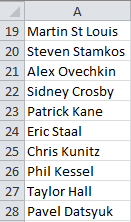
Example 8

=COUNTIF(A19:A28,”P*”)

In this example, it will count the names that start with the letter P. Because the criteria start with P and is followed by an asterisk, what this means is that the first letter has to be a P, and the rest can be anything (three cells match this criteria)

Similarly:

=COUNTIF(A19:A28, “*P”)

This formula works the opposite way, in that it will count the cells where P is the last letter, and any values can come before (no cells meet this criteria).

And also:

=COUNTIF(A19:A28, “*P*”)

This formula will count the cells where P is anywhere in the cell (the same three cells that matched Example 8 are the only ones true here as well).

Note: the criteria here is not case sensitive.

But what if you are only looking for a certain number of characters? For example:

=COUNTIF(A19:A28,”*H???”)

In this formula, it will count names that end with the letter h and 3 characters after. The ? represents one character (cannot be a number). This allows you to control your result to a finite length, whereas the asterisk doesn’t limit the number of characters. The cells that meet this criteria are A21 and A27.

A similar formula:

Example 12

=COUNTIF(A19:A28,”E??c*”)

This formula will look in the range and count the cells that start with the letter e, have any two letters after that, then a c, and anything else after that. The only result in the list is cell A24.