admin, Author at HowtoExcel.net

Free Excel Add-In: 20+ Macros to Automate Tasks and Make You More Efficient

September 10, 2018

by admin with One Comment add-ins lookups macros vba

This add-in is completely free and includes over 20 macros that I have worked on myself and that I hope will help you. Any feedback is welcome, as well as any suggestions for other macros you would like to see added.

Disclaimer
These macros have not been tested exhaustively so I don’t offer any guarantees that they will work under every possible scenario. However, if you run into any issues please let me know and I will work to correct them. When using macros you should always save your work before executing them, as there is no undo button if something doesn’t go as expected.

If you understand and accept these risks, please feel free to download the file here

Below is an overview of all the different macros in the file.

Toggling Workbook and Worksheet Calculations

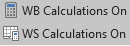
For those that work on large spreadsheets, this can make it easy for you to not only turn off and on calculations for a workbook, but for individual worksheets. It will also allow you to see whether or not they are set to on or off.

One of the things people sometimes don’t realize is if you turn off calculations in Excel at the workbook level, that disables it for all other workbooks. The danger is if you switch to another file you’re working on you may not realize calculations are still off, by seeing the toggle and whether it is set to on or off can help prevent that.

If you only need an individual worksheet to be off, you can do that as well. However, note that if the workbook calculations are set to off, then all the worksheet calculations will be off as well, regardless of whether or not they say on or off. Workbook settings will supersede any worksheet settings.

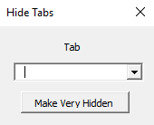
Very Hidden Tabs

Hiding tabs in Excel may seem pointless since even an average user would know that you can right-click and select un-hide. However, not many know that you can set them to be ‘very hidden’ and where right-clicking won’t do anything.

I’ve covered this in a post before here, and in this add-in I’ve made it so that you can easily both hide and unhide very hidden tabs.

Removing Excess Spaces

This macro will delete any trailing, leading, or extra spaces in a cell and will help to clean up your data.

Converting Formulas to Values

In some instances you may want to get rid of your formulas and replace them with their results (values), this macro will do that for you. Just select the cells and click the button and the formulas will be gone.

Converting Numbers to/from Text and Changing Signs

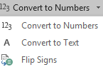
These buttons will allow you to choose whether you want to convert numbers that are stored as text into numbers, switch numbers back into text, or just flip the signs from positive to negative or vice versa.

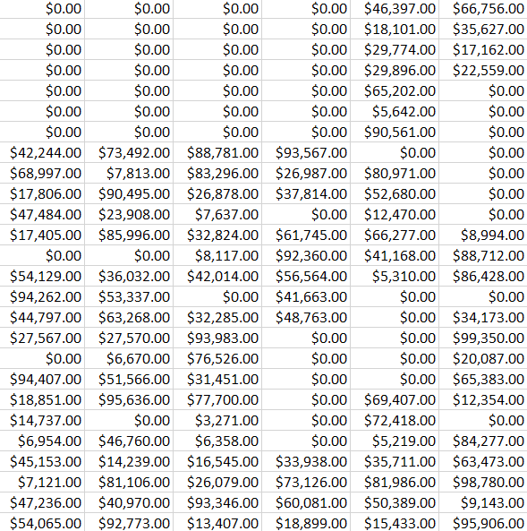
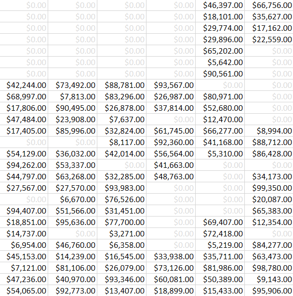
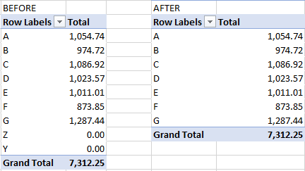
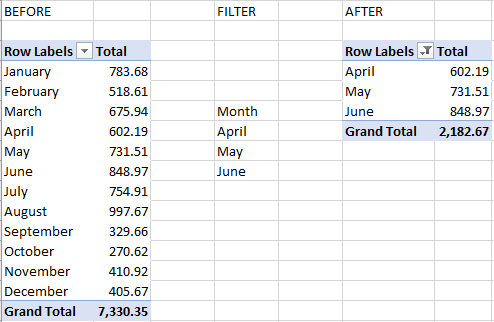
Filtering Out Zero Values From Tables

If you’ve got a table or pivot table that has a lot of zero values in it that you don’t want to see, this will filter them out. This won’t get rid of errors, just zeros, and for it to work in a table, it assumes that the table will start in column A, otherwise it won’t filter the right column for you. The zero values will be removed from the column where your active cell is, so you have to make sure you’ve got the right cell selected before clicking this button.

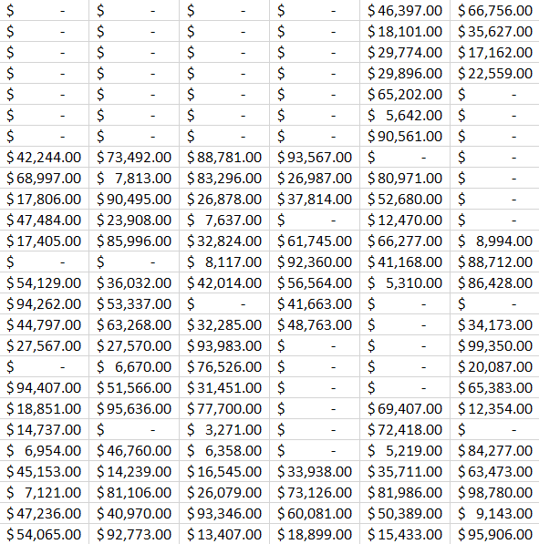
Multiplying and Dividing by a Factor of 1,000

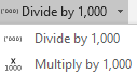
This is pretty straightforward and is mainly here since dividing can be helpful if you’re dealing with financials and want to cut down the number of placeholders. Multiplying will simply undo those changes.

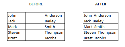
Combining Columns

If you have data across multiple columns and want to combine it, you can do that with this macro. You don’t have to select entire columns, it can just be a selection. The columns don’t even have to be right next to one another.

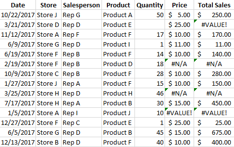
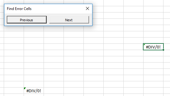
Cycling Through Errors

If you want to find all the errors on the worksheet you’re on, this macro will cycle through all of them for you. You can correct an error, and click the Next button to go onto the next error in the sheet.

Removing Merged Cells

When you’re trying to do data analysis, merged cells can be a nightmare, and this will unmerge the cells and put the value into each of the cells as well.

Protecting Your Data

This will help convert your sensitive data into a random number preceded by a series of X’s. There’s a post here detailing how that process works.

Filtering Pivot Tables

If you’ve got a pivot table and want to select multiple items, it can be a tedious process. This macro will allow you to select what selections you want to filter by and apply them for you. But the first cell in the selection needs to match the field name in the pivot table.

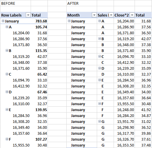
Adjusting the Default Pivot Table Format

One of the more annoying things in Excel is that when you create a pivot table, it defaults to a format that isn’t very useful. This is what the macro will help you do:

Quickly Formatting Pivot Table Fields

If you’ve ever needed to change how fields are formatted in a pivot table you know that simply selecting the column and changing the format is a temporary fix. You need to actually go into the field settings. This macro will do that for you, and will set the settings to either comma or accounting format.

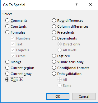
Quickly Extracting Unique Values

There are plenty of ways you can get unique values, but I thought an even easier way would be to select the cells and specify where you want those unique values to be output.

Counting Unique Values

If you just want to quickly count how many unique values are in your selection, this macro will do that for you.

Do a Reverse Lookup

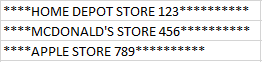
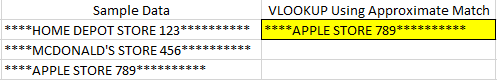
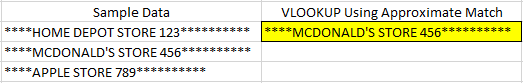
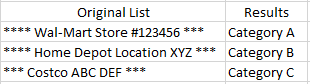
Everyone knows how to do a VLOOKUP, but doing the reverse is another story. Take for example a credit card statement. You could have a lot of detail in the string, but only a certain few characters relate to the actual vendor or detail you want:

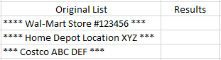
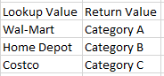
Using this lookup function the cells you select will be compared against a list you have specified, and if there are any matches, the corresponding field will be returned:

The result:

If you’re doing this with a lot of cells and have a big list, it could be time consuming, and that’s why I added a progress bar to this macro.

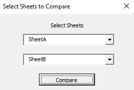
Comparing Sheets

This macro essentially looks at two sheets and tells you what is different, and will highlight the differences in them.

Updating Links

If you want to update the link for a cell, it’s not an easy process and involves you right-clicking on the cell and putting the link in there. This macro will do that step, and for the link it will put the cell’s value there, so if you put in the url you want in the cell and then run the macro on those cells, the links will be updated.

Adding the Location to the Footer

Clicking this button will add the path to the workbook you’re working on into the footer so when you
print it out it’s easy to see where the file is saved.

Using Stacked Charts and Showing Totals

July 28, 2018

by admin with No Comment beginner charts formatting tips & tricks

A stacked chart in Excel allows users to take advantage of the best of both worlds: a column chart that shows period-over-period totals and a pie chart that can show what made up those totals. It can be a very useful chart, but knowing how to structure it is half the battle.

In my example, I pulled Alphabet’s earnings for the most recent four quarters. I wanted to show a) the period-over-period sales as well as where those sales went, and how much flowed through to the company’s operating income.

Below is the table that I used:

The key things is you want to make sure that all your categories add up to the amount that you’re trying to reconcile (in my case, it’s revenue).

Once the data is ready, select the data and insert a Stacked Column

In my example, the categories showed on the horizontal axis, which is not what I wanted, so in order to fix that, right click on the chart and press Select Data

From there, you want to hit the button to switch row/column:

This will give you a stacked chart. The problem, however, is that my total (revenue) is mixed into this, and that’s not going to give me the desired result. After all, I want to see where the revenue goes, not include the revenue in my categories.

To fix this, you’ll want to right click on one of your column charts and select Change Series Chart Type

That should take you to the Combo section. If it doesn’t, make sure to select it. All your series should show a stacked chart. You’ll want to change the revenue series to a Line chart. By doing so, it will not contribute to the stacked chart and now it’ll simply be made up of the other categories.

Next, add data labels for the line chart so now you’ll see the totals. To do this, right click on the line chart and click Add Data Labels

The problem is the labels show to the right, and it probably makes more sense for these labels to show above the stacked chart. Right click on any of the labels and select Format Data Labels

Make sure that for the label position, Above is selected

Now my chart is starting to come together:

Except I still have that line going over the top of the stacked charts. To get rid of the line, right click on the line chart and select Format Data Series

Select No line from the Line section

Now, select the Marker and make sure the fill option is set to No Fill

Now, I’ve gotten rid of the line completely:

At this point it just comes down to designing the chart how you want it. Some of the changes I made included:

Getting rid of ‘Revenue’ from the legend
Changing the color theme
Shrinking the gaps between the stacked charts

Formatting and Removing Errors and Zero Values

July 21, 2018

by admin with One Comment beginner errors formatting iferror match tips & tricks vlookup

Often times in a data set you’ll have to handle with errors that can wreck your data, especially if you need to do any analysis on it. There are several ways that you can handle errors so that they don’t show up in your data.

IFERROR

The first method is by using the IFERROR function, which allows you to easily replace the error with whatever you want in its place. If you want a numerical value, you may want to put in a 0, otherwise you can just leave it blank.

I’ve purposely added various types of errors to my data set:

Here is one of the formulas that’s causing an error:

=VLOOKUP(D7,L:L,1,FALSE)

In the above example, I could use the formula =IFERROR(VLOOKUP(D7,L:L,1,FALSE),””) to replace the error with a blank. I could also put a 0 in its place instead of the “”.

ISERROR

In older versions of Excel (2003 and earlier), the IFERROR function is not available. However, what you can use is a combination of the IF and ISERROR functions. To recreate the same formula as above, we can use the following:

=IF(ISERROR(VLOOKUP(D7,L:L,1,FALSE)),””,VLOOKUP(D7,L:L,1,FALSE))

The disadvantage of this method is you have to repeat your original argument. First, you are checking if the value is an error, if it isn’t, then you have to repeat the formula again to save the value. It’s not terribly efficient, and likely why we saw the IFERROR function introduced in newer versions of Excel.

Using the IFERROR or IF(ISERROR()) functions can be useful for eliminating errors, but sometimes it may not be helpful for dealing with specific ones. For example, if your cell is blank or it has an error and is made to look blank, you won’t be able to tell the difference just by looking at it. The danger is that you may assume it’s a different type of error.

ISNA

What you can also use is the ISNA() function, which can tell you if the cell returns the #N/A error. This way you can trap this error specifically, rather than everything that can be captured by the ISERROR() function.

Getting Rid of Zeros

If you’ve used a lot of error-handling functions and replace your errors with zeros, you could up with a lot of zero values on your spreadsheet:

The problem if you have a lot of zeros on your spreadsheet, is it can sometimes be a distraction away from what you really want to see – the non-zero values. There are two ways you can get rid of the eyesore:

1. Change the format to Accounting. Doing this will remove the zero values and replace them with a dash, which makes it a bit easier to skip over when doing a review:

However, you may not want to use the Accounting format, and that leads me to the other option:

2. Conditional Formatting. Refer to this post on how to setup rules for this. What I normally do in these cases is set the zero value cells to a light gray color font so that they do not attract your attention:

Common Types of Errors

Here’a list of some of the common types of errors you’ll find in Excel:

#REF: This is an error that you’ll incur if your range doesn’t go far enough and the error relates to your reference. For example, consider a VLOOKUP formula that extracts from column number five but you only specified a range that had four columns, that would result in a REF# error.

#N/A: You’ll get this error if your VLOOKUP or MATCH formula is correct, but the value you’re looking up isn’t found, and hence, not available. However, there’s other contexts it can apply to, and it just means that it wasn’t able to find the value you were looking for.

#VALUE: This error normally shows up when there is an issue with your actual calculation. For instance, if you’re trying to multiply a number by a field that has text.

These are just a few examples of the errors that you’ll encounter, but these are also likely the most common that you’ll come across.

Finding Partial Matches and Using Wildcards with VLOOKUP

July 1, 2018

by admin with No Comment intermediate tips & tricks vlookup wildcards

If you’re looking up data, often times just using a VLOOKUP function can be enough to get you your desired result. Sometimes, however, it doesn’t do enough, especially if you’re looking for a partial match.

While you can set VLOOKUP to pull an approximate match rather than an exact match, that may not provide you with the desired results, especially if you’re using text.

Consider the following situation where you’ve got a series of charges from your credit card statement and want to find a particular vendor:

In the above example, let’s assume I’m looking for McDonald’s and do a regular VLOOKUP and set the approximate match argument to true, my formula looks like this:

=VLOOKUP(“MCDONALD’S”,B:B,1,TRUE)

And the result I get is this

As you can see, it’s not what I was hoping for. Excel can’t figure out that I’m looking for the second result, and simply gives me the last one.

Using Numbers with the Approximate Match

The approximate match isn’t useless in VLOOKUP, in fact, when it comes to numbers, it can be very accurate.

Consider the following example:

If I want to find out the tax bracket that a given income level relates to, I’ll use this formula

=VLOOKUP(G11,D:E,2,TRUE)

Assume column D is the taxable income and column E is the tax bracket %, with the taxable income I input being in cell G11.

Using this formula, if I put an income of $0 in G11, my tax bracket is correctly returned as 0%. It’s not until I enter $25,000 that it will return 10%.

Excel understands numbers better than words, and so it knows that since $24,999 is not greater than or equal to $25,000, that it still belongs in the first tax bracket, the one that was 0% and started at $0.

If I enter $105,000 as my income amount, then it also correctly knows that I’m in the 25% tax bracket since that is the highest bracket in the list.

If, however, I don’t put the brackets in the correct order my results won’t be the same. In order for this type of calculation to work, you need to start from the lowest value to the highest.

How Can We Get Text to Work?

If you want your partial text matches to work, you’ll want to use wildcards. What you can do is add an asterisk before and after your search term, which will then return even a partial match. Here’s an example of how the updated formula might look from the first example:

=VLOOKUP(“*MCDONALD’S*”,B:B,1,FALSE)

This might look a bit confusing since now I’m actually not looking for an approximate match, but rather an exact one, as indicated by the FALSE argument at the end.

But because the asterisks will grab everything before and after my text, technically I do want it to match exactly, since it’ll search for my string as well as anything before and after it.

The result:

*Note that the formula is not case sensitive. Whether I type in MCDONALD’S or mcdonald’s, it would have no impact on my result.

As you can see, now I get the partial match that I was looking for. The danger, however, is that your partial string isn’t unique enough. If I were to use the word STORE as my string, I would get the first result that is a match, and in this case that would not be what I want.

Because VLOOKUP will return the value for the first time there was a result, you want to ensure its not a common string that will be found more than once.

Extracting the Largest and Smallest Values in a Dataset

June 14, 2018

by admin with No Comment intermediate large max min small

Retrieving the maximum and minimum values is done relatively easily in Excel using the MIN() and MAX() functions, but what if you wanted to extract the five largest or smallest values?

Two lesser-known functions can help you achieve this: SMALL and LARGE. Both functions work the same way and have the same arguments: (array, k)

In the first argument (array), you select the data you want to pull your value from, and the second argument (k) is how large or small it is with respect to the data (e.g. a value of 5 would give you the fifth largest or smallest value, depending on whether you are using the LARGE or SMALL function).

You could recreate the MAX and MIN results by placing a value of 1 in the second argument, for example:

=SMALL(A:A,1) would return the smallest (minimum) value in column A
=LARGE(A:A,1) would return the largest (maximum) value in column A

However, the real value in using the SMALL and LARGE functions is being able to pull the next smallest, or largest number.

You can use the ROW() function to help you do this.

If you needed to pull the 10 largest or smallest values from a range of data, rather than manually changing the k values manually, what you can do is use the ROW() function, and use ROW(A1) in the first argument and then drag the formula down.

The relative references will change the value to A2, A3, A4, etc. Now whether you use A or B or C as the column doesn’t matter since the formula is only going to calculate the row number.

The formulas might look something like this, assuming you data is in column A:

=SMALL(A:A,ROW(A1))

=SMALL(A:A,ROW(A2))

=SMALL(A:A,ROW(A3))

The value for ROW(A1) is 1, and for ROW(A2) it is 2, so you can see how just by dragging this formula down you can easily increment your formula and pull the next largest or smallest number.

The above example would get you the three smallest values in the data set, whereas the following would return you the three largest:

=LARGE(A:A,ROW(A1))

=LARGE(A:A,ROW(A2))

=LARGE(A:A,ROW(A3))

Are Your Excel Files Too Big? 3 Ways You Can Bring Them Down in Size

May 28, 2018

by admin with No Comment formatting intermediate tips & tricks

If you’ve got a big Excel file (e.g. more than 10 mb) and you don’t have tens of thousands of rows, you may want to see what you can do about bringing that size down.

If you have lots of data, you may want to consider linking it using PowerPivot, although that’s a topic for a future post.

If your Excel file is unnecessarily large and you’re not sure why, there are three things you can do and check for to bring it down in size.

1. Check for objects

If you copied data from a webpage or somewhere that had images, you could have objects on your spreadsheet without ever realizing it. Many times they’ll appear invisible.

This has happened to me before and there’s a quick way to check and delete them if you do have them. Simply click F5, select Special, and then select Objects and hit OK.

If there aren’t any in your sheet you’ll get a message that none were found. If you don’t get that message then clicking delete will remove those that are on the sheet.

This will only look on the individual sheet you’re on so you may want to try this on all your sheets just to make sure.

2. Removing excess rows.

This on many cases is the culprit. People move data around and formatting is left behind and Excel holds data sometimes until the very last row. Again, this is an invisible problem that you won’t easily spot.

What you can do to determine if you have this problem is click on a cell in your data set somewhere and click CTRL + END. This will take you to the very bottom of your data. If it stops where it should, then you’re fine. If it takes you several thousand rows farther than you expect, or worse – to the bottom, then there’s a good chance you’ve found what’s making your spreadsheet all that bigger.

To fix the problem, select the rows from the very bottom all the way up to your last row. Delete these rows and then click save. The file size won’t update until you click save.

Tip: if you have lots of worksheets to go through, user CTRL + PG UP/PG DOWN to cycle through the different sheets and then hit CTRL + END on each one and you can quickly see if any sheet has the problem.

3. Remove unneeded columns

If you really just have too much data, consider deleting excess columns. While in many cases people think of removing unneeded rows, they neglect the impact that columns have. If you’ve got tens of thousands of rows, even deleting one column will remove that many data points. Multiply that by how many columns are unnecessary and the data savings will quickly add up, and your file size will see a noticeable decrease.

These are three of the most common reasons your file might be bigger than it needs to be. Often times people think having a macro is going to do it, but that’s not the case. Usually it’s just having lots of data and doing calculations on all that data will take a big chunk of your computer’s resources

Protect Your Sensitive Excel Data with This Template and Add-in

May 4, 2018

by admin with No Comment add-ins template

One of the challenges sometimes with sending your spreadsheet to someone, whether it’s to review or to make changes to it, is that it contains sensitive information.

So I’ve created a template and add-in that will help you accomplish that.

You can download the template here or if you prefer, the add-in is available here.
Disclaimer: I do not offer any guarantees or promises that this will work perfectly and it’s the responsibility of the user to ensure and confirm that all data is adequately protected as the spreadsheet still requires manual steps from the user.

The template will look like a regular spreadsheet, but with one main difference. On the far right end of the Home tab, you’ll see this button:

If you select the data you want to encrypt, whether it’s a few cells or an entire column, then clicking this button will mask your data. Here’s how it works.

In my spreadsheet, in column A, I have a list of customer names that I want to protect.

If I highlight the range and click on the Encrypt Selection button, what will happen is it will mask the data and create a new tab showing me which customer is mapped to which mask:

After all, masking the data is great, but if you don’t know what the data means, it’s not very helpful. The macro creates a tab called “Mapping Hidden Cells” and it’ll give you a popup warning you to delete this tab before you send the data to anyone. The purpose of this tab is to give you the table, and you can either make note of it or save it somewhere. Either way, you’ll want to delete this afterward, otherwise it would make masking the data pointless.

If I return to my main tab I notice that the data is now masked:

The customer names are now nowhere to be found. At this time I’d like to point out that the masking will only happen to the cells that you selected. If for example I had customer data in a different area and didn’t select it, that data would not have been masked.

This is why it is crucial for the user to review the data themselves and validate that the sensitive information has in fact been correctly masked, and that the mapping tab has been deleted.

5 Useful Excel Shortcuts That Are Underutilized

April 29, 2018

by admin with No Comment beginner shortcuts tips & tricks

There are a lot of ways you can speed up data entry and analysis in Excel, and while most people know about copying and pasting and how to undo actions, there are some useful ones that many users aren’t familiar with.

This list will go over five lesser-known, but useful shortcuts.

1. CTRL + 1 : Formatting cells.

If you find yourself changing the formatting of cells often then using this shortcut could help save some time rather than right clicking format cells. It may not be a huge time saver but if you’re not using the mouse then it’s an easier way to access that menu.

2. CTRL + F1 : Toggle the ribbon

When you’re working with a lot of data often times you’ll need just a bit more space, and hiding the ribbon can help give you see more rows on your page. You can also double-click on the active tab’s name and it will accomplish the same result.

3. CTRL + ~ : Show formulas

If you’re editing a spreadsheet and want to quickly find where there are formulas versus which cells are hard-coded, this is an easy way to show you what is actually entered in the cell, as opposed to what the end value is. The ~ button is normally located next to the 1 on your keyboard.

4. CTRL + ] and CTRL + [ : Showing dependents and precedents

These shortcuts are useful because if you click on a cell that has a formula you can see if there are other cells that are dependent on the cell for inputs somewhere else, or which cells feed into this one. CTRL + [ will show you which cells the active cell depends on, and where its inputs come from, while CTRL + ] will show you if the active cell is used in calculations elsewhere.

You can hit tab to cycle through all the cells that have been highlighted.

It will not show you all the cells if the related cells span multiple tabs, but it can be helpful when looking at formulas and inputs in all other cases.

5. ALT + F1 : Insert a chart

This shortcut can allow you to quickly launch a chart based on the data that you’ve selected. This again may not be a big time saver, but if you’re on a different tab or

Dynamically Filter Data Using Only a Formula

April 22, 2018

by admin with No Comment advanced arrays filter index

In my previous post I went over advanced filters in Excel. This time around I’ll go over how to achieve the same result using just a formula. No macros, no VBA, just through a not-so-simple formula that can dynamically update based on your selections.

I’m again going to use my sample database file for this example. Here’s an excerpt of what that looks like:

Filtering based on one criteria

I’m going to start by filtering all that entries for a specific sales rep.

First, I’m going to use the INDEX function to select the range from where I’m pulling data from.

=INDEX(SampleDatabase!$A$1:$G$1000

For my results, I’m going to want them to show up in the order they appear in the database. For example, in the excerpt above Rep D shows up on lines 3 and 5, and I want that same order to stay intact.

In order to do this, I’m going to use the IF, SMALL and ROW functions, which will be inserted in the INDEX function.

SMALL(IF(SampleDatabase!$C$1:$C$1000=$I$2,ROW(SampleDatabase!$A$1:$A$1000),””),ROW(A1)),1)

$C$1:$C$1000=$I$2 : In this argument, assume that $I$2 is where I have my sales rep name, in this case it would be Rep D. Because I’m only interested in rows that relate to Rep D, this is the main argument that I want to evaluate.

ROW(SampleDatabase!$A$1:$A$1000), “”) : This will return the row number if the above argument is true. It doesn’t matter whether I reference column A, B, C or any other since I’m only pulling the row number. If it isn’t a match, the result will be a blank value.

ROW(A1) : This returns a value of 1, and what this will accomplish is that it will pull the smallest row number from the above list. For instance, for Rep D we know that lines 3 and 5 will be a match, but the smallest number, or the first time that there is a match, is 3. As I drag this formula onto subsequent lines, the row number, because it isn’t frozen, will change and on line 2 it will pull the second smallest row number, on the third line it will be the third smallest, and so on.

The last argument is which column you want to extract. I left it as 1, and that will return the date since that is the first column in my INDEX argument. However, if I wanted to pull the total sales, I could change that to 7, since that would indicate column G, which is the seventh column in the data set that I specified.

The completed formula will look as follows:

=INDEX(SampleDatabase!$A$1:$G$1000,SMALL(IF(SampleDatabase!$C$1:$C$1000=$I$2,ROW(SampleDatabase!$A$1:$A$1000),””),ROW(A1)),1)

This formula will need to be entered as an array, so be sure to hit CTRL+SHIFT+ENTER.

The first five results look as follows:

The one caveat is that if you don’t know how many entries you’ll have and copy the formula down too far, you’ll inevitably end up with #NUM! errors because the formula has not found any more matches. What you can do in this case is use the IFERROR function and include it in the formula:

=IFERROR(INDEX(SampleDatabase!$A$1:$G$1000,SMALL(IF(SampleDatabase!$C$1:$C$1000=$I$2,ROW(SampleDatabase!$A$1:$A$1000),””),ROW(A1)),1),””)

What this will do is now show a blank value if there are no more matches.

Filtering for multiple criteria

While it’s nice to be able to filter for just one criteria, what if you wanted to look for the entries with multiple conditions? Although this makes our already long formula even longer, it is still possible.

Much of the formula stays the same, and the key to making it work is by changing the first argument in the IF statement. Previously, It was only looking for the Sales Rep to be a match:

$C$1:$C$1000=$I$2

I’ll add another criteria, this time for records that include Product E, and I’ll put the product criteria in the cell below in I3. I will add the following to the formula:

$D$1:$D$1000=$I$3

How I combine the two arguments is by multiplying them by one another:

($C$1:$C$1000=$I$2)*($D$1:$D$1000=$I$3)=1

I add the =1 at the end because if both conditions are true then they will result in a 1 value for that line. For example, in the first condition it will look at whether the sales rep is a match, if it is the value will be true (or 1), and if not, it will be false (or 0). The same will happen if the product matches.

Therefore, if either one of those conditions is false then a 0 will be returned and the two conditions multiplied against one another will not equal 1.

Below is how the new formula looks:

=IFERROR(INDEX(SampleDatabase!$A$1:$G$1000,SMALL(IF(($C$1:$C$1000=$I$2)*($D$1:$D$1000=$I$3)=1,ROW(SampleDatabase!$A$1:$A$1000),””),ROW(A1)),1),””)

You’ll notice much fewer matches in column L (multiple criteria) than in column J where I was only looking for the sales rep to be a match.

If you go back to the original excerpt I showed, you’ll see that for the 3/21/2017 entry, it was for both Rep D and Product E. If I change the values in column I then my calculations will adjust accordingly.

How to Use an Advanced Filter

March 10, 2018

by admin with No Comment filter intermediate

There are many ways you can filter data in Excel, and in this post I’ll cover the Advanced Filter.

Using the Advanced Filter will allow you to set a criteria in place for your filter and then put the results in a separate section or tab. The benefit from a normal filter where you select your criteria using drop downs is that it won’t affect the rest of the data.

If you want to follow along with my example, I have the sample database file that I’m going to use available here.

Filtering the Data Using One Criteria

First up, I’m going to look at Sales Rep A’s sales for Product A.

For the Advanced Filter to work, there are two sections that need to be ready: the criteria, and the extract.

For the criteria, you need to have the fields that you want for your filter entered. In my example I only am looking for Rep A’s Product A sales, so I only enter that criteria and don’t enter any other fields.

In the extract section, which you’ll see just below the criteria section above, I enter the fields I want to see. I don’t have to list all the fields, just the ones that I want to see. Please note the field names need to be an exact match with those in your data set. If they are not, the filter will not work as expected.

Now, to execute the Advanced Filter I’ll click on the Advanced button that is under the Data tab next to the Filter button.

After doing so, you’ll be prompted to enter two sections:

In the List range you want to enter your table, or the data you want to filter. In the Criteria Range you will select the fields you want to filter along with the criteria you want to match.

You can either Filter the list, in-place which will effectively do the same job as if you filtered your data using the drop down options. If you select Copy to another location then the third field, Copy to, will be available for input and this is where you will select your extract fields.

These are what my inputs look like:

After I click OK, my results are as follows:

This looks the same as if I were to filter using the drop down, but the benefit is I am effectively copying the data to another location.

Using Multiple Criteria

In the previous example, I used an Advanced Filter just using one set of criteria. In this example, I’ll add another to create a more complex filter.

When using the criteria in an Advanced Filter, if criteria are on the same line it is the same as using the AND operator, while if the criteria are on different lines it is the equivalent of using OR.

In the first example, Rep A and Product A were on the same line, meaning that my criteria was that it had to be Rep A and Product A. In the following example, I’m going to add another criteria:

The above criteria says that it will look for Rep A’s Product A sales OR Product B when Total Sales are more than $500.

When I re-run the Advanced Filter, I’ll have to expand my range to include the new criteria:

The results:

The results are either Product A or B, and B only shows up when the Total Sales are more than $500. You can add even more criteria, you’ll just need to expand the criteria range when running the Advanced Filter.

Copying to Another Sheet

In both of these examples I’ve copied data over within the same tab. However, if I wanted to copy it to another sheet, that is possible as well.

To do this, you’ll need to copy the headers you want for the extract into another tab. You need to press the Advanced Filter button on the tab where you want the data extracted to. So if you create another sheet, it’s on that sheet that you’ll need to press the button for the filter to work.

In addition to the headers, you’ll also need to put something in the second row, as the Advanced Filter button will result in an error if there is only one row of data when you click on the button (when you first use it). If there was data there before it should be fine, but the very first time you move data over you might get an error message if there isn’t data on the second row.

Once your headers are properly setup, you run the Advanced Filter button and fill in the same data as before. The one difference you’ll see is that since I’m on a different tab, the sheet name will show up in the Criteria and List range fields:

Generating a Unique List of Values

There are a lot of different ways you can pull a list of the unique values in a list. Excel has even added a button to remove duplicates, but it will remove the other items in your list, so that may not be ideal.

The Advanced Filter will allow you to do this as well, simply by just leaving your criteria blank and checking off the box for Unique records only

If I want to generate a unique list of Salespersons, I’ll run the Advanced Filter with these options:

The result:

Because I only wanted to see the unique values for the Salesperson, I only have that field in my extract list.

Benefit of Using the Advanced Filter

At first glance, you may be wondering why even bother with an Advanced Filter. After all, you can setup the filters yourself using drop downs and then copying and pasting the filtered data somewhere else.

The most likely reason for the Advanced Filter is that in earlier versions of Excel, filtering just wasn’t as strong as it is today.

The main benefit using it today is that it can allow you to easily audit and trace your filters. If you just copy and paste after applying filters you won’t be reminded of which filters you put in place.

If you use older versions of Excel you’ll likely find a lot more usefulness out of the Advanced Filter than if you are using the newer versions. Admittedly, I haven’t had a need to use the Advanced Filter in several years and can’t imagine that changing anytime soon.