functions – HowtoExcel.net

How to Use the CHOOSE Function in Excel: A Comprehensive Guide

May 27, 2025

by howtoexcel functions

When it comes to working with Excel, mastering the various built-in functions can save you time, increase your efficiency, and unlock new ways to analyze your data. One such function, often underutilized but incredibly powerful, is the CHOOSE function, which is available in Excel 2016 and newer versions. In this guide, I’ll explain what the CHOOSE function does, how to use it, and provide you with practical, real-world examples to help you become an Excel power user.

What is the CHOOSE Function in Excel?

The CHOOSE function in Excel allows you to select a value from a list of options based on a given index number. It’s like a simplified version of a lookup function: you specify a number, and Excel returns the corresponding value from a set of choices you provide.

Why Use the CHOOSE Function?

Quickly pick from a list of options without complicated formulas.
Useful for creating drop-down dependent formulas, simple scenarios, or mock data.
Combines well with other functions to create flexible, dynamic formulas.

CHOOSE Function Syntax

The syntax of the CHOOSE function is as follows:

=CHOOSE(index_num, value1, [value2], …)

index_num: The position number in the list of values you want to return. This must be a number between 1 and 254.
value1, value2, …: The possible choices (up to 254 in total).

Example:

=CHOOSE(2, “Red”, “Blue”, “Green”)

Result: Blue

Explanation: The index number is 2, so Excel picks the second value, which is “Blue”.

Basic Examples of the CHOOSE Function

Let’s start with some simple use cases to help you understand how CHOOSE works.

Example 1: Picking a Day of the Week

Suppose you have a number between 1 and 7 and want to return the corresponding weekday.

Using the choose function in excel to select a day of the week.

If cell A1 contains 1, the formula returns “Sun”

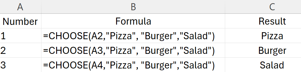
Example 2: Creating a Simple Menu

You want to return a meal based on a number.

Using the choose function in excel to select a menu item.

Practical Uses for CHOOSE in Excel

Now that you’ve seen the basics, let’s explore how the CHOOSE function can help you solve real-world Excel problems.

1. Simulating a VLOOKUP with CHOOSE

Although VLOOKUP is often used to look up values, you can use CHOOSE to create a two-way lookup, especially for dynamic scenarios.

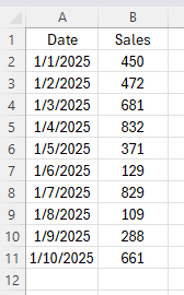
Example: Dynamic Lookup Table

Suppose you have sales data for two years in columns:

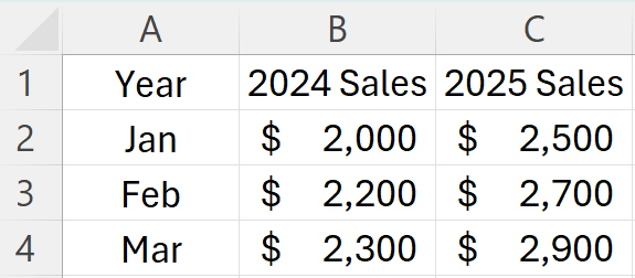
Using the choose function in excel to select a sales value.

You want to pick which year’s sales to show based on a cell (say, cell D1: 1 for 2024, 2 for 2025).

Formula in cell D2:

=CHOOSE($D$1, B2, C2)

If D1 = 1, you see sales for 2024.
If D1 = 2, you see sales for 2025.

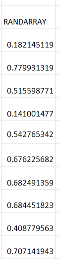
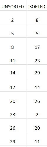
2. Generating Random Items from a List

Combine CHOOSE with the RANDBETWEEN function to randomly pick an item.

=CHOOSE(RANDBETWEEN(1,3), “Apple”, “Banana”, “Cherry”)

Each time you recalculate, Excel picks one fruit at random.

3. Creating Conditional Labels

Suppose you have a grading system:

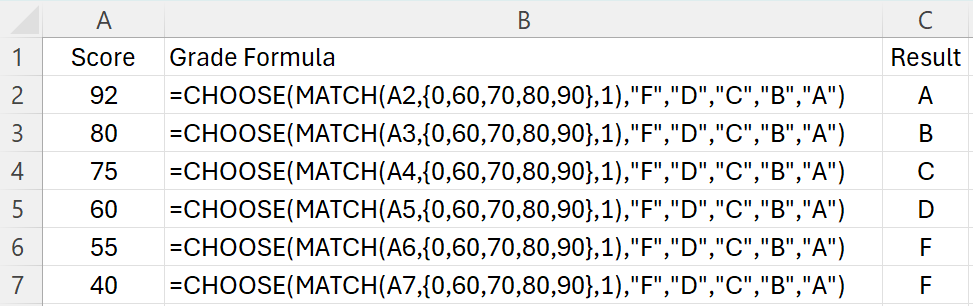
Using the Choose function to lookup grades.

MATCH returns a number 1-5, which CHOOSE uses to assign “F”, “D”, “C”, “B”, or “A”.

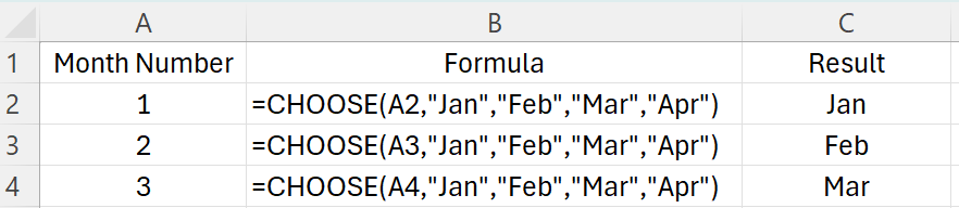
4. Working with Dates

Pick the correct month, quarter, or label based on a number.

Using the Choose function to lookup a month value.

Combining CHOOSE with Other Functions

The true power of CHOOSE comes when you combine it with other functions for advanced scenarios.

Example: Dynamic Chart Series

You have two data series and want to switch which series your chart displays using a dropdown (Data Validation).

Set up your options in a cell (1 = Sales, 2 = Profits).
Use CHOOSE to dynamically reference your data:

=CHOOSE($B$1, SalesRange, ProfitsRange)

Where SalesRange and ProfitsRange are named ranges.

Example: Returning Ranges

You can return entire ranges with CHOOSE (useful in array formulas or dynamic charts).

=SUM(CHOOSE(2, B2:B10, C2:C10, D2:D10))

Returns the sum of column C.

Common Errors and Troubleshooting

1. #VALUE! Error

Reason: The index number (index_num) is less than 1 or greater than the number of choices.
Solution: Check that your index number is within the valid range.

2. #REF! Error

Reason: You are trying to reference a range outside of what is available (for example, referencing a column that doesn’t exist).
Solution: Double-check your value references.

3. Non-integer Index

Reason: Index number is not an integer.
Solution: Ensure the index is a whole number.

CHOOSE vs. INDEX vs. SWITCH: Which to Use?

CHOOSE: Best for a small, fixed list of options, or when returning ranges or arrays.
INDEX: Better for large lists, dynamic lookups, or when referencing ranges based on a row/column number.
SWITCH: Great for exact matching of values.

Example:

Use CHOOSE when you want =CHOOSE(2, “Apple”, “Banana”, “Cherry”) for simple selection.
Use INDEX when you have a table and want =INDEX(A2:A100, 5).
Use SWITCH for matching exact values: =SWITCH(A1, “A”, 1, “B”, 2, “C”, 3, “Other”).

Frequently Asked Questions

Q: Can CHOOSE be used with arrays?
A: Yes, you can use CHOOSE in array formulas, especially to select between ranges for dynamic charts or calculations.

Q: What is the maximum number of choices in CHOOSE?
A: Up to 254 values can be specified.

Q: Can CHOOSE be used with text, numbers, ranges, and formulas?
A: Yes, you can use CHOOSE to return text, numbers, cell references, ranges, or even calculations.

The CHOOSE function in Excel is a versatile, easy-to-use tool that can simplify many tasks, from random selections to dynamic reporting. While it may not replace more advanced lookup functions in every situation, it shines when you need to pick from a small set of options or return specific ranges dynamically.

By mastering CHOOSE, you add another valuable skill to your Excel toolkit, helping you work smarter and faster.

If you liked this post on How to Use the CHOOSE Function in Excel: A Comprehensive Guide, please give this site a like on Facebook and also be sure to check out some of the many templates that we have available for download. You can also follow me on Twitter and YouTube. Also, please consider buying me a coffee if you find my website helpful and would like to support it.

How to Use the PIVOTBY Function in Excel

May 6, 2025

by howtoexcel functions pivot table

PIVOTBY is a relatively new function that Excel introduced in 2021. It is a dynamic, formula-based alternative to pivot tables. It’s part of Excel’s push toward more dynamic, flexible data analysis, especially for users who prefer formulas over the drag-and-drop interface of traditional PivotTables. In this article, I’ll walk you through what PIVOTBY does, how to use it, and provide some examples to help you master it.

What Does the PIVOTBY Function Do?

PIVOTBY summarizes data based on one or more grouping columns and returns an array with calculated values—similar to a pivot table, but directly inside a formula.

It allows you to group data by categories (like region, product, or date) and then apply an aggregation function (like SUM, AVERAGE, COUNT, etc.) on another column. Here are the main arguments for the function:

PIVOTBY(row_fields,col_fields,values,function,[field_headers],[row_total_depth],[row_sort_order],[col_total_depth],[col_sort_order],[filter_array],[relative_to])

Only the first four arguments are required:

row_fields: this the range which will be used to group rows.

col_fields: this is the range which will group the columns.

values: this is a range for the data which is to be aggregated.

function: this determines how the data should be aggregate (e.g. SUM, AVERAGE, COUNT)

How the PIVOTBY Function Works

Here’s a sample data set that I am going to use to illustrate how the PIVOTBY function works:

Excel table showing expenses by department and employee.

In the above table, dates are in column A, the name is in column B, followed by store in column C, department in column D, and amount in column E. Assuming my data is in a table called tblData, I can use the following syntax to create a pivot table showing sales by name and store:

=PIVOTBY(tblData[Name],tblData[Store],tblData[Dollar Amount],SUM)

This produces the following values:

Summary of values generated in Excel using the PIVOTBY function.

If you want to turn off totals for the rows, then you can set the row_total_depth argument to 0, as is the case below:

=PIVOTBY(tblData[Name],tblData[Store],tblData[Dollar Amount],SUM,,0)

And if you want both column and row totals off:

=PIVOTBY(tblData[Name],tblData[Store],tblData[Dollar Amount],SUM,,0,,0)

You can also pull in multiple columns or rows with the help of the CHOOSE function. Suppose you wanted to pull in both the name and the department a person is from. Here’s how you can accomplish that, while also removing totals:

=PIVOTBY(CHOOSE({1,2},tblData[Name],tblData[Department]),tblData[Store],tblData[Dollar Amount],SUM,,0,,0)

This produces the following report:

Pivotby report showing expenses by employee, department, and store.

The benefit of this setup is that since this is a spill function, it will automatically update and populate the data and no refresh is necessary. There are, however, downsides to consider:

If there is not enough space for the pivot table, you will encounter a #SPILL! error.
Unlike a conventional pivot table, you can’t drill down to see the details
This won’t work on versions of Excel prior to 2021.

If you just want an easy way to summarize your data without the need for drilling down, then the PIVOTBY function can work well and be a suitable replacement for a normal pivot table. For more of a comparison between the function your typical pivot table, check out this video:

If you liked this post on How to Use the PivotBy Function in Excel, please give this site a like on Facebook and also be sure to check out some of the many templates that we have available for download. You can also follow me on Twitter and YouTube. Also, please consider buying me a coffee if you find my website helpful and would like to support it.

How to Use the TRIMMEAN Function in Excel

April 21, 2025

by howtoexcel average averages functions

What is the TRIMMEAN function?

The TRIMMEAN function has been available on Excel since the 2016 version. What it does is return the mean (average) of your data set, but it excludes a portion of your data. This can be useful if you want to exclude outliers and data that may not be typical. Small and large numbers can sometimes skew a data set and while you could use the MEDIAN function to get the middle value, you may also prefer to just exclude the highest and lowest values.

It offers another way to calculate an average, which may be more representative than the MEDIAN. What you may want to consider is using the function alongside the MEDIAN and AVERAGE functions, to see just how much of a disparity there is in your data set.

How the TRIMMEAN function works

The TRIMMEAN function has just two required arguments: array and percent. The first argument is the array of numbers you want to calculate for the average. The second argument is where you specify the percentage of outliers you want to exclude. If you have 10 data points and enter 0.2 for 20%, that would eliminate 2 data points — 1 from the top and 1 from the bottom.

In the below example, I have a list of 10 random numbers between 1 and 100:

A list of 10 random numbers in Excel, showing the results of the AVERAGE and TRIMMEAN function.

Using the AVERAGE function, it calculates a value of 32.9 as the average. But if I apply the TRIMMEAN function as specified above, where I exclude 20% of the values, then the value I get is 31.5. Here’s how that is calculated:

Random numbers averaged in Excel when excluding the largest and smallest values.

If you sort the data and exclude the largest and smallest number, the rest will average out to 31.5. If I were to change my percentage argument to 0.4 and 4 numbers are excluded, the top 2 and bottom 2 numbers will be excluded:

But what if the percentage you specify doesn’t result in an even number to remove from the top and bottom? For example, what if you want to exclude 30% of the numbers from a list of 10 values? In that case, the TRIMMEAN function still excludes just 2 numbers. Until it can remove an even number from both the top and the bottom, it won’t exclude any further numbers. Here’s how it calculates as you increase the percentage:

How the TRIMMEAN function calculates in Excel at varying percentages.

As you can see, the TRIMMEAN function doesn’t return a different amount until it gets to 40%, at which point it can remove an even numbers from the top and bottom of the range (2).

This is an important thing to keep in mind when using the function as it can result in an incorrect assumption that you are ignoring a certain percentage of numbers when really, it won’t be excluding that many unless you enter a high enough percentage where it can trim an equal number from the top and bottom of the range.

How does this compare against the MEDIAN calculation?

The big question is whether this TRIMMEAN function is still useful given the noted limitations. Here’s how it calculates versus the MEDIAN function, which simply takes the middle number (or averages the two middle values):

How the TRIMMEAN function calculates in Excel at varying percentages compared to the MEDIAN.

In this example, the TRIMMEAN function returns a lower value. However, if the values 47 and 48 and changed to 37 and 38, then the result would be as follows:

The MEDIAN function is the only one which returns the same value, since it is averaging the middle two values (30 and 35). However, both the AVERAGE and TRIMMEAN functions return lower values.

There is no right or wrong function to use but using all three can help you gain some insights into your data and how much variance there is in it.

If you liked this post on How to Use the TRIMMEAN Function in Excel, please give this site a like on Facebook and also be sure to check out some of the many templates that we have available for download. You can also follow me on Twitter and YouTube. Also, please consider buying me a coffee if you find my website helpful and would like to support it.

How to Generate a List of Non-Repeating Random Numbers in Excel

April 8, 2025

by howtoexcel functions random

Do you want to create a list of random numbers in Excel, but avoid repeating values? Below, I’ll cover how you can set that up to ensure that no number is shown more than once — all through just a single formula.

Start with the SEQUENCE function

The first thing that’s necessary is to create a list of numbers to choose from. It needs to be in the form of an array, which can then be sorted. Using the SEQUENCE function, I can create an array which goes from 1 to 10 with the following formula:

=SEQUENCE(10,1)

The first argument specifies the rows to fill in, and the second one is the number of columns. If you wanted to start from the number 2 and jump by 3 values at a time, the formula would be as follows:

=SEQUENCE(10,1,2,3)

This produces the following, unsorted list:

List generated by using the sequence function in Excel, which starts from the number 2 and jumps by 3s.

The next step is where the numbers get reordered. Another array of numbers needs to be created. This time, I’ll use the RANDARRAY function, since I want the array to be entirely random. I will again need to specify the number of rows and columns to fill in:

=RANDARRAY(10,1)

This produces a list of random numbers, similar to how the RAND function works. The only difference is that it creates a list for you:

Using the RANDARRAY function to create an array of random values.

Next, let’s combine these two formulas, within the SORTBY function. With the SORTBY function, you can specify the range you want to sort, and how you want it to be sorted. The complete formula is displayed as follows:

=SORTBY(SEQUENCE(10,1,2,3),RANDARRAY(10,1))

And this will now sort the sequence randomly. Here is the sorted and unsorted sequence, side by side:

Unsorted and randomly sorted columns in Excel.

The column on the left, shows the unsorted values, as they have been created with the SEQUENCE function. The column to the right, however, has applied a random sort with the help of the RANDARRAY and SORTBY functions. The values are randomized and do not repeat. If you want to re-sort them, you just need to trigger a recalculation. This can be done by just pressing the delete key on any cell.

For this to work, both arrays have to be sized the same. In both functions, 10 rows and 1 column are used. However, if they are not the same size, the formula will produce an error. You could decide to have 1 row and 10 columns to display the values horizontally, with the following formula:

=SORTBY(SEQUENCE(1,10,2,3),RANDARRAY(1,10))

This will produce a randomized list which goes horizontally:

At this stage, you could use this random list as is or you could also combine it with a lookup function to extract a certain item based on a pre-defined value.

If you liked this post on How to Generate a List of Non-Repeating Random Numbers in Excel, please give this site a like on Facebook and also be sure to check out some of the many templates that we have available for download. You can also follow me on Twitter and YouTube. Also, please consider buying me a coffee if you find my website helpful and would like to support it.

How to Use the TRIMRANGE Function in Excel

April 1, 2025

by howtoexcel functions trim

Microsoft Excel has recently rolled out a new function, TRIMRANGE. And as its name suggests, it will help you trim a range, to ensure that your formula is efficient and isn’t including unnecessary blank values in calculations. Here’s a breakdown of the function.

The inputs for the TRIMRANGE function

There are three arguments to enter for the TRIMRANGE function:

Range: the range that you want to trim.

Trim_Rows: specify which rows to trim from the specified range. 0=no rows; 1=leading blank rows; 2=trailing blank rows; and 3=both leading and trailing blank rows (this is the default).

Trim_Columns: specify which columns to trim from the range. 0=no columns; 1=leading blank columns; 2=trailing blank columns; 3=both leading and trailing blank columns (default).

If you just want to trim everything, then you don’t need to worry about entering any arguments beyond just the initial range you want to trim.

How to function works

In the following example, I have values filled in only up until row 11:

With the TRIMRANGE function, I can select the entire range A:B, and it will return an array of the values which only contain values. The formula only requires that one range.

=TRIMRANGE(A:B)

This is the result:

If, however, there are gaps within the data set, then it will return zero values:

Result of the TRIMRANGE function when there are gaps within the range.

Where it performs well is when it excludes leading and trailing empty spaces:

Result of the TRIMRANGE function when there are gaps before or after a range.

If you like this post on How to Use the TRIMRANGE Function in Excel, please give this site a like on Facebook and also be sure to check out some of the many templates that we have available for download. You can also follow me on Twitter and YouTube. Also, please consider buying me a coffee if you find my website helpful and would like to support it.

Use Excel’s Image Function to Populate Logos

January 28, 2025

by howtoexcel functions

The IMAGE function in Excel is one of the newer ones you can use. And it can make importing images into your spreadsheet a whole lot simpler than saving, uploading, and then inserting them. I’ll also show you how to setup a template where you can dynamically import logos from a website.

How the Image function works

The main ingredient for the IMAGE function is the URL of the image you want to use. This means you no longer have to save an image you want to use. All you need to do is to point to where it is found online. Suppose, for example, I want to insert Netflix’s logo into my sheet. I can look for the logo online, and then copy the URL into the formula’s first argument:

=IMAGE(“https://upload.wikimedia.org/wikipedia/commons/thumb/7/7a/Logonetflix.png/1200px-Logonetflix.png”)

This will now display the Netflix logo in the cell:

By expanding the cell, the image will automatically expand. It will do so in accordance with its dimensions.

Other arguments in the IMAGE function include the following:

Alt_Text: this is what will show if the image cannot be displayed.
Sizing: this determines how the image should be displayed and contains the following options:
- Fit Cell: This is the same as the default behavior, where it will expand based on the size of the cell, while maintaining its true dimensions.
- Fill Cell: This will fill the cell as much as possible and may result in the image stretching.
- Original Size: This will be based on the original image’s size; no scaling will take place and if the image is very large, it may not fully display in the cell.
- Custom Size: A custom size needs to be set in the height and width arguments.

The simplest option is to simply leave the default options, allowing the image to automatically expand based on the size of the cell. This ensures the image is not stretched out and gives you a lot of control over how it is displayed, without worrying about setting custom dimensions.

Creating a formula to populate logos

You can create a formula which will dynamically adjust based on your inputs, and pull in different images accordingly. Suppose you wanted to pull in logos for companies. You could do that by using a website such as logo.clearbit.com. The site has links to images based on their domains. While it may not work in the future, the way it’s linked gives you an idea of how this can be setup.

For example, the URL https://logo.clearbit.com/netflix.com will link to an image for Netflix. Different domains will show different images. If I setup a formula which connects the IMAGE function and starting URL along with a domain, I can make this dynamic so that the logos will update based on the domains I input.

=IMAGE(“https://logo.clearbit.com/”&B1)

The above formula will use the IMAGE function and combine the clearbit URL along with what I have entered in cell B1. And if that’s set to a domain, the image will update accordingly. Here’s how the formula works with multiple examples:

Image function in Excel pulling in different logos based on their domains.

The formulas are in column A and rely on the values in column B to create the full URL, which includes the clearbit site along with the domain. The end result is an easily updatable function which pulls in images based on my entries in column B.

You can create a similar type of setup if you host images on a site. By creating consistent names for your images, you can use them within the function so that you can easily point to the images you want.

If you like this post on How to Use Excel’s Image Function to Populate Logos, please give this site a like on Facebook and also be sure to check out some of the many templates that we have available for download. You can also follow me on Twitter and YouTube. Also, please consider buying me a coffee if you find my website helpful and would like to support it.

Calculate Interest Savings on a Credit Card Balance Transfer in Excel

June 18, 2024

by howtoexcel functions personal finance

A balance transfer for a credit card allows people to move the outstanding balance from one or more credit cards to a new card, often with a lower interest rate. The purpose of a balance transfer is to reduce the amount of interest paid on existing debt, which can help cardholders save money. Many credit card issuers offer promotional periods with significantly reduced interest rates, sometimes as low as 0%, for a specified duration, typically ranging from six months to 18 months.

By transferring high-interest credit card balances to a card with a lower or 0% interest rate, cardholders can save a substantial amount of money on interest payments. For example, if an individual has a $5,000 balance on a card with a 20% annual percentage rate (APR), they would accrue approximately $1,000 in interest over a year. However, if they transfer that balance to a card offering a 0% APR for 12 months, they can avoid paying any interest during the promotional period, allowing them to allocate more of their payments towards the principal balance.

Additionally, a balance transfer can simplify debt management by consolidating multiple balances into one monthly payment. This can make it easier to keep track of payments and avoid missed or late payments, which can result in additional fees and negatively impact one’s credit score. However, it’s important to be aware of balance transfer fees, which typically range from 3% to 5% of the transferred amount. Even with these fees, however, the potential interest savings often outweigh the cost, making balance transfers an attractive option for those looking to manage their debt more effectively.

In the example below, I’ll show you how an Excel spreadsheet can help you estimate just how much you might save with a balance transfer.

Calculating credit card interest savings in Excel

You can estimate the interest savings from a balance transfer in Excel using the future value (FV) function. The function takes multiple arguments:

Interest Rate
Number of Periods
Payment Amount
Present Value
Payment Type (beginning or end of period)

Since we are looking at monthly payments, we will need to convert the interest rate to a monthly percentage. For this, take the annual credit card rate and divide it by 12. If your credit card charges a 20% interest rate annually, dividing that by 12 will give you a monthly percentage of 1.67%. In Excel, this would be input as 0.0167.

The number of periods would represent the number of months. If it’s a six-month promotional period, then six would be your input, 12 if it’s for 12 months, and so on.

As for the payment, let’s suppose that you will pay 3% of the balance. On a $1,000 credit card balance, that would translate into a monthly payment of $30.

For the present value, we’ll enter a negative value to indicate an amount owing. The input will be -$1,000.

The last argument, for the type of payment, can be left blank, assumes that a payment will be made at the end of the period. By setting it to a 1, that will assume the payment is made at the beginning. For the purposes of estimating, however, this won’t have a significant impact on the calculation.

The complete formula for the calculation based on the above assumptions for a 12-month period is as follows:

=FV(0.2/12,12,30,-1000)

This returns a value of $824.49. This is what the balance would be after 12 months of payments. Next, let’s compare this to what the balance would be if the interest rate was 0%. This what that formula would look like:

=FV(0,12,30,-1000)

This returns a value of $640, and it’s the same as if you were to deduct $360 (12 payments of 30) from the balance. Thus, the savings from the balance transfer, before accounting for fees, would be:

824.49 – 640.00 = 184.49

Furthermore, let’s assume there is a 4% balance transfer fee. On a $1,000 balance, that would be $40. The final cost savings would be as follows:

184.49 – 40.00 = 144.49

This is just one example of a savings calculation, but let’s adjust this so that it is more adaptable to other scenarios, and create a template which can be easily modified.

Creating a template to calculate savings from balance transfers

With the logic setup, to create a template is just a matter of determining the inputs to plug into the calculation. The variables which a user should be able to adjust are as follows:

The current interest rate
The promotional rate
The monthly payment amount
The credit card balance
The promotional period in months
The balance transfer fee

For this example, I’m going to use much larger amounts to help emphasize the potential savings. These are the inputs I’ve created in my sheet:

Excel sheet with inputs for credit balances and interest rates.

Now, it’s a matter of setting up the formula which links to these values. To do this, we need to combine the following calculations:

The FV based on the current credit card interest rate,
The FV based on a 0% credit card interest rate
Calculating the difference between the two FV calculations
Deducting the balance transfer fee from the above calculation

The first FV calculation is a copy of what was used before, except this time the values are not hardcoded and are instead linked back to the input cells above:

=FV(B1/12,B5,B3,-B4)

For the second FV calculation, we just need to reference the promotional rate:

=FV(B2/12,B5,B3,-B4)

Then, we deduct the difference between these calculations:

=FV(B1/12,B5,B3,-B4)-FV(B2/12,B5,B3,-B4)

The following formula also factors in the balance transfer fee:

=(FV(B1/12,B5,B3,-B4)-FV(B2/12,B5,B3,-B4))-(B6*B4)

Assuming a $20,000 credit card balance, with a monthly payment of $600, an interest rate of 20%, a 12-month promotional period at 0%, and a 4% balance transfer fee, the total cost savings would be approximately $2,889.74. The completed template is setup as follows:

Cost savings calculation in Excel showing the benefits of a credit card balance transfer.

By setting up this template in Excel, you can adjust these inputs to do your own what-if analysis. These calculations assume that your credit card balance does not change and that you are simply paying it down and not adding to it.

If you like this post on How to Calculate Interest Savings on a Credit Card Balance Transfer in Excel, please give this site a like on Facebook and also be sure to check out some of the many templates that we have available for download. You can also follow me on Twitter and YouTube. Also, please consider buying me a coffee if you find my website helpful and would like to support it.

Amortization calculator which calculates values for a specific period.

Create an Amortization Calculator in Excel

March 12, 2024

by howtoexcel accounting amortization calculator functions

Amortization schedules are essential tools for anyone managing a loan or mortgage, providing a clear breakdown of how payments are allocated towards interest and principal over the loan’s term. Typically, these schedules detail each payment’s date, the interest portion, the principal portion, and the remaining balance, offering borrowers insight into the precise cost of borrowing over time. Creating an amortization schedule in Excel can be a time-consuming process, but with the help of some advanced payment functions, you can expedite the process and even eliminate the need for creating an entire amortization table.

Generating the key components of an amortization schedule

Whether you’re creating a full-blown amortization schedule or just want to calculate the balance at a future point in time, you’ll need to know the following values before you can begin:

the loan value,
the interest rate and compounding,
the number of periods, and
the start date of the loan

Suppose you have a $500,000 loan with a 5% interest rate, which is for a period of 10 years, and that payments are made on a monthly basis. Given this information, you can start by calculating the monthly payment amount. Here’s what the inputs would look like for the PMT function:

=PMT(0.05/12,10*12,-500000,0) = 5,303.28

This assumes compounding to be monthly, hence the need to divide the interest rate by 12. And the negative 500,000 balance tells the function that this is an amount owing and that it will reduce over time. The following argument, 0, is to signify that the future value is 0.

There is also an additional argument, for whether the payments are made at the beginning or the end of the period. The default is set to the end of the period. If payments are made at the beginning, then the final argument is set to 1. If the payment is at the start, then the payment value would change to $5,281.27, assuming all the other values remain the same. But for the purposes of these examples, we’ll assume payments are made at the end of the period.

Creating a calculator for specific month’s calculations

Now that you have all the necessary variables, including the payment amount, you can start to create the calculator.

In this first case, we’ll look at how to calculate values for just a specific period. Let’s assume the loan’s start date is January 1, 2024. And let’s assume we want to calculate what the balance, interest, and principal payment amount will be for the month of Dec 2025.

How to calculate amortization amounts for a specific period:

1. Start with calculating the period number. One function that can help with this is the DATEDIF function. By using it, you can quickly calculate the difference between two time periods. Here’s how it would work in this example:

=DATEDIF(“1/1/2024″,”12/1/2025″,”m”) = 23

Two full years have not fully elapsed until we get to 1/1/2026. But since we want to calculate the values for the 24th month, we’ll need to add 1 to the equation. The formula to calculate the current period will be as follows:

=DATEDIF(“1/1/2024″,”12/1/2025″,”m”)+1

2. Calculate the interest payment for the period. To get the interest amount, use the IPMT function:

=IPMT(0.05/12,24,120,-500000) = 1,760.19

3. Calculate the principal amount paid down during the period. In this case, we can use the PPMT function. It is the same setup as the previous formula:

=PPMT(0.05/12,24,120,-500000) = 3,543.08

4. Calculate the ending value as of that period. Using the FV function, here’s the formula to get the ending balance as of the end of Dec 2025:

=FV(0.05/12,24,5303.28,-500000) = 418,902.68

By using these functions, you no longer need to make an entire amortization schedule. You can simply do a calculation for the period you need to sum up the values for. By creating inputs for the start of the loan, loan amount, interest rate, # of periods, and the period you want to calculate for, you can setup an amortization calculator as follows in Excel:

Calculate amortization values for a specific range

Suppose you wanted to calculate the interest and payment values for all the months in 2025. This can be a bit trickier since we aren’t calculating amounts for just a single period anymore. Instead, we need to get a range of values.

How to calculate amortization amounts for a specific multiple periods:

Step 1. Get the correct period numbers. Let’s assume the loan began on June 1, 2023. We need to get the starting period number, which is Jan. 1, 2025. This can be done with the DATEDIF function:

=DATEDIF(“6/1/2023″,”1/1/2025″,”m”)+1 = 20

This tells us that January is the 20th month of the loan. If January is the 20th month, then that also means if we add 11, that December will be the 31st month of the loan. Thus, our range of periods is 20 through 31. You could, however, use the DATEDIF function to do the calculation for that period as well.

Step 2. Calculate the interest payments for the year. Now that we know the periods we need to calculate the interest for, we can use the CUMIPMT function:

=-CUMIPMT(0.05/12,120,500000,20,31,0) = 20,851.88

The present value cannot be set to negative for the cumulative function, or else you will get an error. To adjust for this and avoid a negative value, simply add a dash before the function to ensure the result is flipped from a negative value to a positive one.

Step 3: Calculate the total of the principal payments made during the period. To calculate the principal paid during the period, we can use the CUMPRINC function. The inputs are the same as that of the cumulative interest payment calculation:

=-CUMPRINC(0.05/12,120,500000,20,31,0) = 42,787.43

Step 4. Get the ending period’s balance. Just as with the previous section, we can use the same FV calculation to get the ending balance. This time, it will be for period 31.

=FV(0.05/12,31,5303.28,-500000) = 393,684.23

Here is how the calculator could be setup to make these calculations based on a range.

Amortization calculator which calculates values for a specific range.

You can download the amortization calculator I have created from these examples here.

If you liked this post on How to Create an Amortization Calculator in Excel, please give this site a like on Facebook and also be sure to check out some of the many templates that we have available for download. You can also follow us on Twitter and YouTube.

How to Calculate Running Totals in Power Query

February 6, 2024

by howtoexcel functions power query

Do you have year-to-date values and need to calculate running totals? What about if you have criteria you want to track running totals for? In this post, I’ll show you how to accomplish both and how you can create a custom function in Power Query that you can re-use in other queries. Here is a simple table I am going to use for this example:

Table in Excel showing sales by day, rep, and location.

In this table we have date, sales, salesperson, and location. Initially, I am just going to calculate the running total, regardless of the salesperson. I just want to know how much everyone has generated up to a certain point in time. The one step that I need to do is sort the dates in order, so they are going from smallest to largest. You can do this in either Excel or within Power Query.

Creating a running total for everything in Power Query

Step 1: Load your data into Power Query

To load your existing table into Power Query, click on your table and select the Data tab and click on From Table/Range.

Selecting the From Table/Range button in the Data tab.

Step 2: Sort your data

If your data is not already sorted in Power Query, then select the Date column and click the button to sot in ascending order.

Step 3: Create an Index column

On the Add Column tab, select the option to insert an Index Column, and select to the option to start From 1:

Creating an index column in Power Query.

This now creates a simple column that starts from 1.

A Power Query table with an index column.

Step 4: Create a column for the Running Total calculation

Select the Custom Column button from the Add Column tab, which will let you create a column based on a formula.

Selecting the Custom Column button from the Add Column tab.

There are two functions will be used in the formula. The first is the List.Sum function, which as the name describes, will sum up the values in a list. Within that will be the List.FirstN function which will grab all the index values up until that point. The custom column formula to enter, is as follows:

=List.Sum(List.FirstN(#"Added Index"[Sales],[Index]))

This is how it appears within the Power Query screen:

Creating a formula for a custom column in Power Query.

This now creates a Running Total column which calculates the year-to-date sales values:

A Power Query table after adding a Running Total column.

Creating a running total for when criteria is met in Power Query

This time around, I’m going to show you how to create a running total which resets for each salesperson. By doing this, you can track their individual year-to-date totals. If you’re starting from scratch, you will need to repeat the steps from the previous section in order to arrive at your Running Total formula.

Step 1: Convert the Running Total formula into custom function

Once you have created the Running Total formula, you can convert it into a custom function. If you select the query and click on the Advanced Editor button on the home tab, you will see the code for all the steps which were previously created:

Power Query advanced editor showing multiple steps.

To reuse this code and use it as a function, I need to add a place to enter a variable at the beginning.

let runningtotal = (x) =>

In the above example, x is the input. It will refer to the table which the custom function will execute on. And at the end of the custom function, there should be another ‘in’ keyword to circle back to the function, such as follows:

in runningtotal

Here is how my custom function looks like after removing the Changed Type step and setting the source equal to the variable:

The advanced editor showing a formula to calculating a running total.

If you remove any steps, however, just remember to update the formulas. In the “Added Index” step, I updated the step I’m referencing to Source. Otherwise, it would reference a step that doesn’t exist and would result in an error.

After saving, you should notice an fx function next to your query, which you may want to now rename to your desired function name. This is what you will reference it to when invoking the function. In this example, I’m going to call it RunningTotal to keep everything consistent.

Now the function is ready to be used.

Step 2: Group the data

On the Home tab, select the Group By button. This will allow you to break your data into multiple tables.

Selecting the Group By button in Power Query.

In the Group By section, select the option to group by Salesperson and use All Rows as the operation, which ensures no data is lost. I’ll name the new column Data.

Grouping data by salesperson in Power Query.

This now creates a column that contains tables based on the salesperson:

Power Query data which has been grouped by salesperson.

Step 3: Invoke the custom function

On the Add Column tab, press the button to Invoke Custom Function

Invoking a custom function in Power Query.

Then, on the details, enter the column name, the function to invoke, and the data which contains the variable. Since the new ‘Data’ column contains the table, that will be the variable in this example. But if you named the column differently, you would use that name.

This will now create an additional column, which also contains a table.

A Power Query table after invoking a custom function to create a new column.

If you click on any of the cells in the newly created field, you’ll see that the preview contains the running total field:

A preview in Power Query of a table nested within a field.

Step 4: Expanding the table

The last step involves expanding the tables in the newly created field. By pressing on the two arrows going in opposite directions, you will be able to expand all of the columns.

You can omit including the Index column as that is not necessary, and the Salesperson field is already there. The only other column you may want to remove in addition to this is the Data column, but that has to be removed with an additional step. Here is how my final table looks:

A Power Query table after adding a field for the running total.

You can see that as the name changes to a different salesperson, the running total doesn’t continue adding; it starts from the first date for that salesperson.

If you liked this post on How to Calculate Running Totals in Power Query, please give this site a like on Facebook and also be sure to check out some of the many templates that we have available for download. You can also follow us on Twitter and YouTube.

Create a Date and Time Stamp in Excel Using VBA

November 28, 2023

by howtoexcel dates functions vba

Do you have a spreadsheet that needs to track dates? Whether it’s a shipping log, an inventory tracker, a sales order template, or just something to track when the last change was made to a cell, there’s an easy way you can create a date stamp in Excel with VBA.

Use checkboxes to make your spreadsheet more user friendly

If you have a spreadsheet where you want to track statuses, using checkboxes can be helpful. This way, someone can check or uncheck the status of an order. This can indicate whether it has been shipped, ordered, or completed. Excel has made it easier to insert checkboxes with a recent update. If you’re using Microsoft 365, then on the Insert tab on the Ribbon, you should see an option to insert a Checkbox:

Selecting to insert a checkbox into Excel.

When you click on this button, it will insert a checkbox right into the active cell that you’re on. Want to insert checkboxes into multiple cells at once? Simply select a range of cell and then click on the button:

If a checkbox is checked, its value is TRUE. If it is unchecked, then the value is FALSE. This is important to know when creating formulas.

Populating the date using the NOW() function isn’t useful for date stamps

If you want to enter the current date into a cell, you can use the CTRL+; shortcut. The problem is that it won’t change if you go to uncheck and re-check a checkbox. It’s a stale value and it isn’t a formula.

What you may be tempted to use is the NOW() function. However, the limitation here is that anytime the cell recalculates, it will refresh with the current date and time. It won’t hold the existing date stamp. You can create a circular reference and adjust iterative calculations. But there’s an easier way you can create a date stamp in Excel with just a few lines of code using VBA.

Creating a custom function using VBA

You can create a custom function with VBA. To do, start by opening up your VBA editor using ALT+F11. On the Insert menu, select the option for Module. There, you’ll have an empty canvas to enter code on. The custom function can simply contain one argument — the cell that contains the checkbox. This is to determine whether it is checked (TRUE) or unchecked (FALSE). If it is checked, then the timestamp will be equal to the current date and time. If it’s unchecked, then the timestamp will be blank, and so will the cell value.

Here’s the full code for the function:


Function timestamp(checkbox As Boolean)

    If checkbox = True Then
        
        timestamp = Now()
    
    Else
    
        timestamp = ""
    
    End If
    

End Function

This function is now created. To use it within your spreadsheet, all you need to do is select a cell where you want the date and time to populate on. Then, assuming your checkbox is in cell A2, enter the following formula:

=timestamp(A2)

This will run through the VBA code to determine whether to populate the current date and time or not. Since there is no NOW() function present in this formula, it won’t recalculate with the current date.

Formatting your date and time

Even if the custom function work, you may notice that the value that it populates doesn’t look right. If you get a number or the time is missing from the date, then you’ll need to modify the cell format. To do that, select the cell and press CTRL+1. Then, select the Date category where you’ll see various date formats:

If you scroll down the list, there will be an option that shows the date and time:

If you use that format, then your date will now look correct, including both the date and time.

If you like this post on How to Create a Date and Time Stamp in Excel Using VBA, please give this site a like on Facebook and also be sure to check out some of the many templates that we have available for download. You can also follow me on Twitter and YouTube. Also, please consider buying me a coffee if you find my website helpful and would like to support it.