
Microsoft Excel has recently rolled out a new function, TRIMRANGE. And as its name suggests, it will help you trim a range, to ensure that your formula is efficient and isn’t including unnecessary blank values in calculations. Here’s a breakdown of the function.
The inputs for the TRIMRANGE function
There are three arguments to enter for the TRIMRANGE function:
Range: the range that you want to trim.
Trim_Rows: specify which rows to trim from the specified range. 0=no rows; 1=leading blank rows; 2=trailing blank rows; and 3=both leading and trailing blank rows (this is the default).
Trim_Columns: specify which columns to trim from the range. 0=no columns; 1=leading blank columns; 2=trailing blank columns; 3=both leading and trailing blank columns (default).
If you just want to trim everything, then you don’t need to worry about entering any arguments beyond just the initial range you want to trim.
How to function works
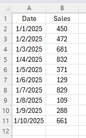
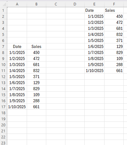
In the following example, I have values filled in only up until row 11:
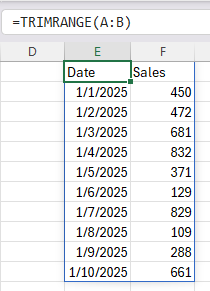
With the TRIMRANGE function, I can select the entire range A:B, and it will return an array of the values which only contain values. The formula only requires that one range.
=TRIMRANGE(A:B)
This is the result:
If, however, there are gaps within the data set, then it will return zero values:
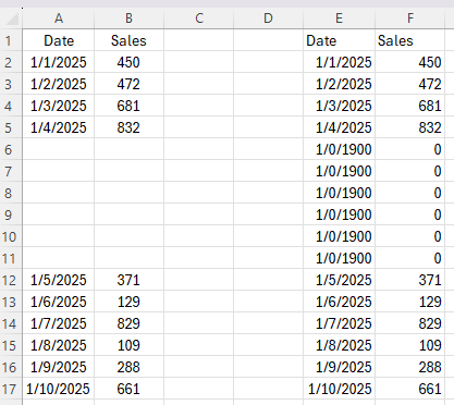
Where it performs well is when it excludes leading and trailing empty spaces:
If you like this post on How to Use the TRIMRANGE Function in Excel, please give this site a like on Facebook and also be sure to check out some of the many templates that we have available for download. You can also follow me on Twitter and YouTube. Also, please consider buying me a coffee if you find my website helpful and would like to support it.