MovingAveragesinExcel

What Is the Difference Between a Moving Average and an Exponential Moving Average

Moving averages can be useful in data analysis, when looking at trends both in finance and in the stock market. You can look at 30, 60, 90 day trends, and even longer or shorter durations. There’s also a difference between whether you are looking at a simple moving average and an exponential moving average. In this article, I’ll go over the differences between the two, and show you how you can calculate them in Excel.

How to Calculate a Moving Average (MA) in Excel

A moving average is a simple tool used by investors and traders to smooth out price data over a specified period. It is called “moving” because it is continually recalculated based on the latest data, providing a dynamic view of an asset’s average price over time. The advantage of an MA is its simplicity as it can easily be calculated.

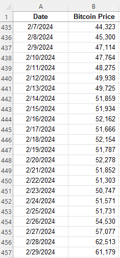
A moving average is calculated by simply taking the average of the trailing periods. In the case of a 60-day MA, you would look at the average over the past 60 days. If it’s a 90-day MA, then you average the past 90 days. In the following example, I have the price of Bitcoin over the past few years. Ideally, when setting up moving averages, you want your dates in ascending order, going from oldest to newest.

Price of Bitcoin in an Excel spreadsheet.

Here are the steps to calculate the moving average:

  1. Determine the number of periods you want to go back. For 5 days, it will be 5, for 10 days it will be 10, and so on.
  2. Calculate the average in the adjacent column. Make sure you do not freeze cells.
  3. Copy the formula down so that the average moves (hence why you do not want to freeze cells).

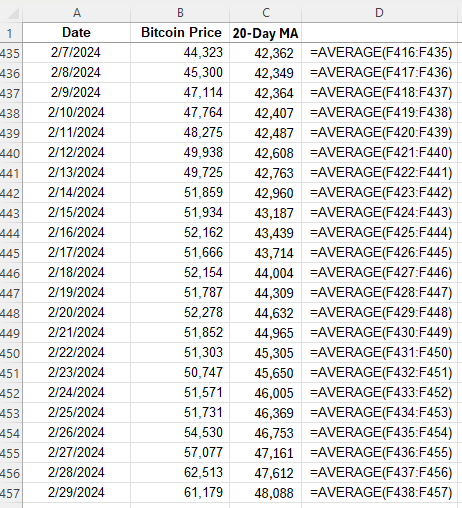
Here is what the values look like, along with the formula for each cell:

20-day moving average of Bitcoin in an Excel spreadsheet.

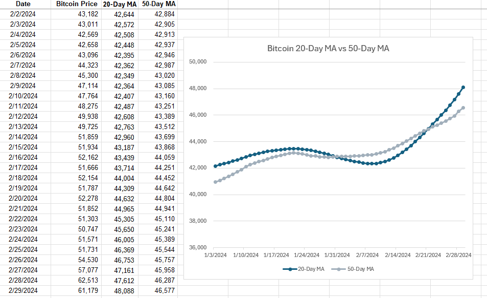
The average is continuously moving with each cell, but it always contains a range of 20 values since the 20-day MA contains 20 days. Oftentimes, people using multiple moving averages as a way to identify crossovers, such as when stocks cross 20-day MAs and 50-day MAs. Depending on the direction of the crossover, it can be a very bullish indicator (20-day MA crosses from underneath) or a very bearish indicator (20-day MA crosses from above). This is what those moving averages look like for Bitcoin and how they appear on a chart:

A bullish crossover involving Bitcoin's 20-day moving average and its 50-day moving average.

In this example, the 20-day MA made a bullish crossover recently, going higher than the 50-day MA. This is a very bullish trend. However, with simple moving averages, these trends can take a while to develop, and that is one of the drawbacks of using them — they are slower to react to recent price movements.

How to Calculate an Exponential Moving Average (EMA) in Excel

The exponential moving average (EMA) gives more weight to recent prices, making it more responsive to new information, and thus, there’s less of a lag effect; changes and crossovers can occur much more rapidly. This characteristic makes the EMA a preferred choice for many traders, especially those looking to capitalize on short-term trends.

Here’s how to calculate an exponential moving average in Excel:

  1. Determine the number of periods, as you did with the simple moving average.
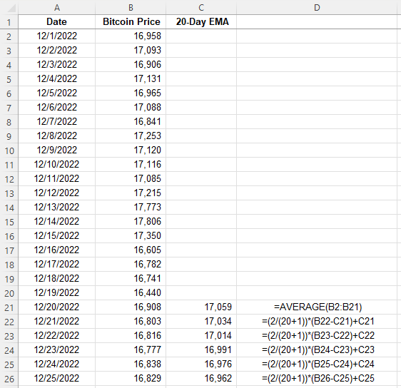
  2. Calculate a multiplier, using the formula 2 / (period +1). In the case of a 20-day MA, the multiplier would be 0.095, which is 2/(20+1).
  3. Calculate the moving average for the first period. The very first period needs to be a simple moving average.
  4. For every value afterwards, you’ll use the following formula: =Multiplier x (Current Price – Previous EMA) + Previous EMA.

Here’s how this would be calculated with the price of Bitcoin, as in the previous example:

Calculating Bitcoin's exponential moving average in Excel.

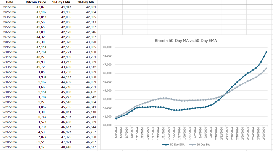
After the initial moving average, the subsequent averages are calculated using the weighting. Here’s a side-by-side comparison of how the 50-day EMA compares with the 50-day MA. I’m using 50-day averages here since they are normally slower to see movements in. But by using an EMA, that can help expedite trends.

Comparing Bitcoin's 50-day exponential moving average against its 50-day simple moving average.

The 50-day EMA makes quicker, more rapid movements and is changing more frequently while the 50-day MA is smoother and more gradual in its changes. With Bitcoin’s price rising rapidly in recent weeks, that uptrend is observed more immediately with the EMA than with the simple MA.

Which Should You Use: MA or EMA?

While both MAs and EMAs provide valuable insights into market trends, the choice between them depends on the specific needs of the trader or analyst. MAs are best suited for identifying long-term trends, as they smooth out price fluctuations evenly. In contrast, EMAs are ideal for those looking to react quickly to recent price changes due to their emphasis on newer data.

By understanding the differences between these two types of averages and knowing how to calculate them in Excel, investors and analysts can better tailor their strategies to suit their goals. Whether it’s the simplicity and broad trend identification of the MA or the responsiveness of the EMA to new information, both tools can be useful.


If you liked this post on What Is the Difference Between a Moving Average and an Exponential Moving Average, please give this site a like on Facebook and also be sure to check out some of the many templates that we have available for download. You can also follow us on Twitter and YouTube.

WeightedAverage

How to Calculate Weighted Average in Excel

A weighted average is a type of average that assigns different weights or values of importance to each element in a dataset. Unlike a simple average that treats all elements equally, a weighted average adjusts the contribution of each element based on its relative significance. This means that some elements have a greater impact on the final result than others, depending on their weights.

Why use a weighted average?

Weighted averages are useful because they provide a more accurate representation of the data by taking into account the importance of each element. For example, in financial analysis, a weighted average may be used to calculate the average interest rate of a portfolio of loans or investments, where the weight of each loan or investment is based on its size or duration. In schools, a weighted average may be used to calculate a student’s overall grade by assigning different weights to assignments, quizzes, and exams based on their importance or difficulty. Anytime you don’t want everything to have the same weighting or importance is when you’ll want to use a weighted average.

Calculating a simple weighted average in Excel

A common way to apply a weighted average is by using a points system. Suppose you are looking to buy a house and have many different criteria that you want to take into consideration, such as square footage, location, if it has a basement, etc. But not all of these items are equally important, and so you may want to say that location is worth 30 points and square footage is worth 25 points, and so on.

The first step is to assign a weight, or point value, to each one of these criteria. Then, assign a score to each one of them criteria, perhaps within a range of 1 to 100. Once you’ve done that, you multiply the score by the points. Total that up, and divide it by the total points, and you’ve got your score, or weighted average. Here’s an example:
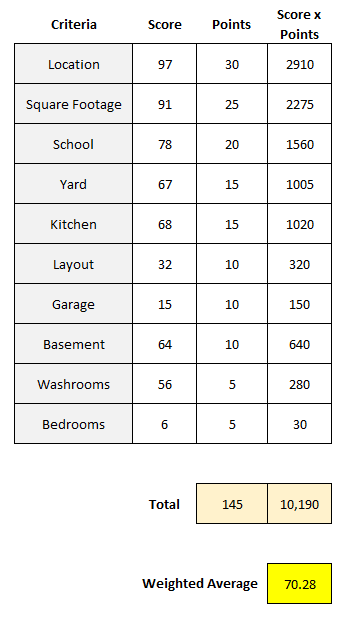
Sample weighted average calculation when evaluating the purchase of a house.

This particular house scored high on the most important items, and thus, resulted in a high weighted average. The total of the score x points column was 10,190. Taking that value and dividing it by 145, the total points, results in a weighted average of 70.28.

Here’s another house, which scores far lower, with a weighted average of just 45.48:
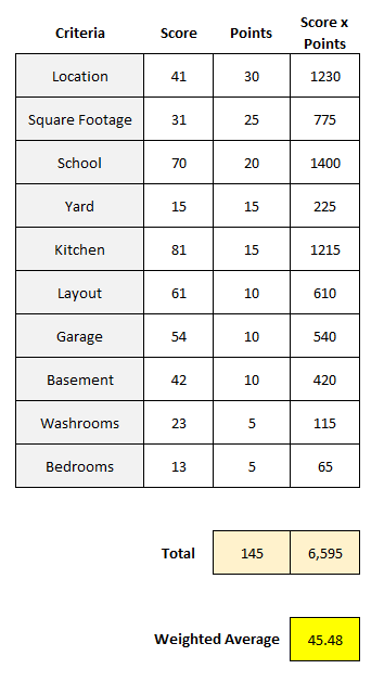
Sample weighted average calculation when evaluating the purchase of a house.

Although it scored high on areas such as school and kitchen, because of its low scores on the top two weightings — location and square footage — that kept its weighted average down.

Creating a template like this in Excel and comparing your different scores can be a way to help compare houses and other things, while giving each criteria an appropriate weighting. By simply scoring everything on a value of 1-100 without weighting, the problem would be that each criteria would effectively be equal, saying that things like layout and the garage are just as important as the location and size of the house, which most people likely wouldn’t agree with. By using weights, you can better take into account the value of each individual criteria.

Calculating grades using weighted averages

Another use for calculating weighted averages is when it comes to grading. In a class, you might have a specific weighting scale that says assignments are worth 10% of your grade, quizzes are 20%, a project is worth 5%, a mid-term is 25%, and the final exam accounts for 40%.

In this case, you’re using percentages that add up to 100% rather than weights, which may be more subjective. This still works in largely the same way as you are multiplying a score by the weight. Except now, since the weights add up to 100%, you don’t need to worry about taking the total and dividing it by the total weights. Whatever your result is, that is the total score. Here’s an example of how a student scored in a class:
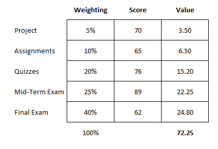
Calculating a student's grade using a weighted average calculation.

When using percentages for weighting, it’s important to double check they add up to 100% to ensure everything is accounted for. In this example, the student had a score of 72.25, which would be the same as saying they scored 72.25%, which would be their grade for the course. As you’ll notice, the student’s high scores on the quizzes and mid-term exam were unfortunately offset by a poor final exam mark.

In this example, since we’re just looking at percentages, you can do without the extra column for value, which takes the weight x the score. Instead, you can use SUMPRODUCT. If the weightings are in cells A2:A6 and the scores are in B2:B6, the grade can be calculated with the following formula:

=SUMPRODUCT(A2:A6,B2:B6)

The formula will multiply each value by the corresponding value in the same row, thereby eliminating the need to use an extra column. By using an Excel formula, you can save yourself the extra step of having to tally up the values and then dividing them by their weights again.


If you liked this post on How to Calculate Weighted Average in Excel, please give this site a like on Facebook and also be sure to check out some of the many templates that we have available for download. You can also follow me on Twitter and YouTube. Also, please consider buying me a coffee if you find my website helpful and would like to support it.

15ExcelAccounting

15 Excel Functions Accountants Should Know

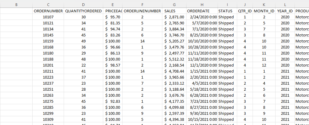
If you’re an accountant, you know that working with large amounts of data can be a daunting task. But with Excel, that work can get a whole lot easier and more efficient. Understanding Excel’s advanced features and functions can improve productivity, reduce errors, make your work more accurate, and most importantly — save you time. Below, I’ll go over some of the most important Excel functions that accountants should know, and provide examples of how to use them. For this example, I’ll use the following spreadsheet. Feel free to download it and follow along with the calculations.

1. SUM

The SUM function is a basic but essential function in Excel. It allows you to add up a range of values, which is helpful when calculating totals, such as revenue, expenses, and profits. Suppose you have a spreadsheet with sales data. In the above example, the total sales are in column G. If you wanted to sum up the entire column, the formula would be as follows: =SUM(G:G)

2. AVERAGE

The AVERAGE function calculates the average of a range of values. It is useful when analyzing data and preparing financial statements. In the above example, suppose you wanted to calculate what the average sale was. To do this, you can just use the AVERAGE function on column G, similar to the SUM function before. Here’s the formula: =AVERAGE(G:G)

3. IF

The IF function allows you to test a condition and return one value if the condition is true and another value if the condition is false. This can be useful because it can send your formulas to the next level. By knowing to use the IF function, you could also use SUMIF, AVERAGEIF, and many other functions that involve an if statement. In the above example, let’s say you only wanted to know if a value in cell M2 was part of the Motorcycles product line. The formula would be as follows: =IF(M2=”Motorcycles”,1,2). If it is part of Motorcycles, you would have a value of 1, otherwise, it would be 2.

4. SUMIF

By knowing the SUM and IF functions, you can combine them together with SUMIF, which is an incredibly popular function. It gives you a quick way to tally up the totals that meet a criteria. For example, let’s say you want all sales that relate to the Motorcycles category. The formula for that would be as follows: =SUMIF(M:M,”Motorcycles”,G:G). If the criteria is met in column M, then the formula will sum up the corresponding values in column G. There’s also the super-powered SUMIFS function, which allows you to combine multiple criteria.

5. EOMONTH

The EOMONTH function calculates the last day of the month for a specified number of months in the future or past. It is useful when working with data that is organized by date. For accountants, this can be useful when you’re calculating when something is due. Let’s say in this example, we need to calculate the date orders need to go out on, and that needs to be the end of the next month. Using the ORDERDATE field in column H, here’s how that calculation would look in the first cell, which would then be copied down for the rest: =EOMONTH(H2,1)

6. TODAY

The TODAY function is helpful for accountants in calculating deadlines and knowing how many days are remaining or past a certain date. Suppose that you wanted to know how many days have past since the ORDER DUE DATE that was calculated in the previous example. Rather than entering in a static date that every day you would need to change, you can just use the TODAY function. Here’s how a formula calculating the days since the deadline for the first cell would look like, assuming the due date is in column N: =TODAY()-N2. The next day you open up the workbook, the calculations will update to reflect the current date; there’s no need to make any changes. There are many more date calculations you can do in Excel.

7. FV

The FV function calculates the future value of an investment based on a fixed interest rate and a regular payment schedule. You can use it to calculate the future value of an investment or savings account. Let’s say that you wanted to save $10,000 per year and expect to earn a return of 5% per year on that investment. Using the FV calculation, you can do that with the following formula: =FV(0.05,5,-10000). If you don’t enter a negative for the payment amount, the formula will result in a negative value. You can also specify whether payments happen at the beginning of a period (1) or end (0 — this is the default) with the last argument in the function.

8. PV

The PV function lets you do the opposite and work backwards from a future value to the present. Knowing that the calculation in example 7 returns a value of $55,256.31, that can be used in the PV calculation to check our work: =PV(0.05,5,10000,-55256.31). The formula returns a value of 0, which is correct, as there was no starting value in the FV calculation.

9. PMT

The PMT function calculates the periodic payment required to pay off a loan with a fixed interest rate over a specified period. It is helpful when determining the monthly payments required to pay off a loan or mortgage. Let’s take the example of a mortgage payment where you need to pay down $500,000 over the period of 30 years, in monthly payments. At a 5% interest rate, here’s what the payment calculation would be: =PMT(0.05/12,12*30,-500000,0). Here again the ending value needs to be a negative to avoid a negative value in the result. And since the payments are monthly, the periods need to be multiplied by 12 and the interest rate is dividend by 12.

10. VLOOKUP

The VLOOKUP function allows you to search for a value in a table and return a corresponding value from another column in the same row. It’s one of the most common Excel functions because of how useful and easy to use it is. It is helpful when working with large data sets and performing data analysis. Let’s suppose in this example that you want to find the sales related to order number 10318. The formula for that calculation might look like this: =VLOOKUP(10318,C:G,5,FALSE). In a VLOOKUP function, you need to specify the column number you want to extract from, which is what the 5 represents. If you’re using Office 365, you can also use the newer, flashier XLOOKUP function. I put VLOOKUP on this list because it’ll work on older versions of Excel — XLOOKUP won’t.

11. INDEX

The INDEX function allows you to return a value from a data set by specifying the row and column number. It’s also helpful if you just want to return data from a single row or column. For example, the sales column is in column G. If I know the order number is on row 20 (which relates to order number 10318), this formula would do the same job as the VLOOKUP in the previous example: =INDEX(G:G,20,1).

12. MATCH

The MATCH function allows you to find the position of a value within a range of cells. Oftentimes, Excel users deploy a combination of INDEX and MATCH instead of VLOOKUP due to its limitation (e.g. VLOOKUP can’t extract values to the left of the lookup field). In the previous example, you had to specify the row belonging to the order number. But if you didn’t know it, you could use the MATCH function within the INDEX function. The MATCH function would look like this: =MATCH(10318,C:C,0). Placed within an INDEX function, it can replace the argument where in the previous example, we set a value of 20: =INDEX(G:G,MATCH(10318,C:C,0),1). By doing this, you have a more flexible version of the VLOOKUP function. You can also create dynamic formulas using INDEX and MATCH that use lookups for both the column and row.

13. COUNTIF

The COUNTIF function allows you to count the number of cells in a range that meet a specified condition. Let’s count the number of values in the data set that are Motorcycles. To do this, you would enter the following formula: =COUNTIF(M:M,”Motorcycles”).

14. COUNTA

The COUNTA function is similar to the previous function, except it only counts the number of non-empty cells. With no criteria, it is helpful to just the total number of values within a range. To calculate how many cells are in this data set, you can use the following formula: =COUNTA(C:C). If there are no gaps in data, then the result should be the same regardless of which column is used. And when combined with the UNIQUE function, you can have an easy way to count the number of unique values.

15. UNIQUE

The UNIQUE function returns a list of unique values within a range, and it’s a much easier method than the old-school way of extracting unique values. If you wanted to extract all the unique product lines in column M, you would enter the following formula: =UNIQUE(M:M). If, however, you just wanted to count the number of unique values, you could embed it within the COUNTA function as follows: =COUNTA(UNIQUE(M:M)). You can adjust your range if you don’t want to include the header.

This is just a sample of some of the useful Excel functions that accountants can utilize. If you are familiar with them, you’ll put yourself in a great position to improve the efficiency of your workflow and make your spreadsheets easier to use. Plus, you can confidently say that you are highly competent with Excel, which can make your resume more attractive and make you better suited for accounting jobs that require advanced Excel skills — and there are many of them that do!.


If you liked this post on 15 Excel Functions Accountants Should Know, please give this site a like on Facebook and also be sure to check out some of the many templates that we have available for download. You can also follow me on Twitter and YouTube. Also, please consider buying me a coffee if you find my website helpful and would like to support it.
adc

Average Down Calculator Template

If a stock you invested in dropped in price, it could be a good opportunity to buy more shares and bring your average down. You can use the average down calculator on this page to do a quick what-if calculation to determine how many more shares you would need to be. However, you can also use this template, which will allow you to run through the same scenarios within Excel.

How the average down template works

There are only six inputs on this template:

  • Amount invested
    • This is how much money you have already invested into the stock.
  • Shares owned
    • The number of shares that you own.
  • Current share price
    • What the share price is.
  • Desired average price
    • What price you want to average down to.
  • Budget
    • How much money you can afford to invest.
  • Increment price by
    • This is for the sensitivity analysis and determines by how much you want it to move by. The default is set to $0.50.

Once you’ve entered that data, the rest of the template will populate. Here are the two scenarios that it will show you:

1. Getting to your desired average price

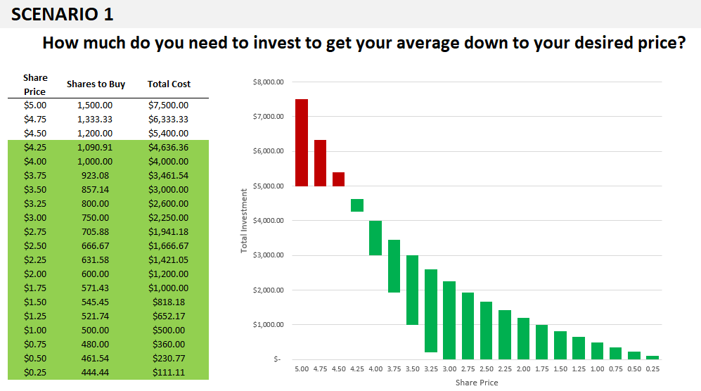
In this scenario, the template will show you how much to invest at different price points to get your average down to your desired average price. You will see up to 20 different data points to show you if the price continues to get lower, how many shares you will need to buy to reach the average price you are targeting.

And any scenarios that fall within your budget will be highlighted in green, and so will the corresponding chart:

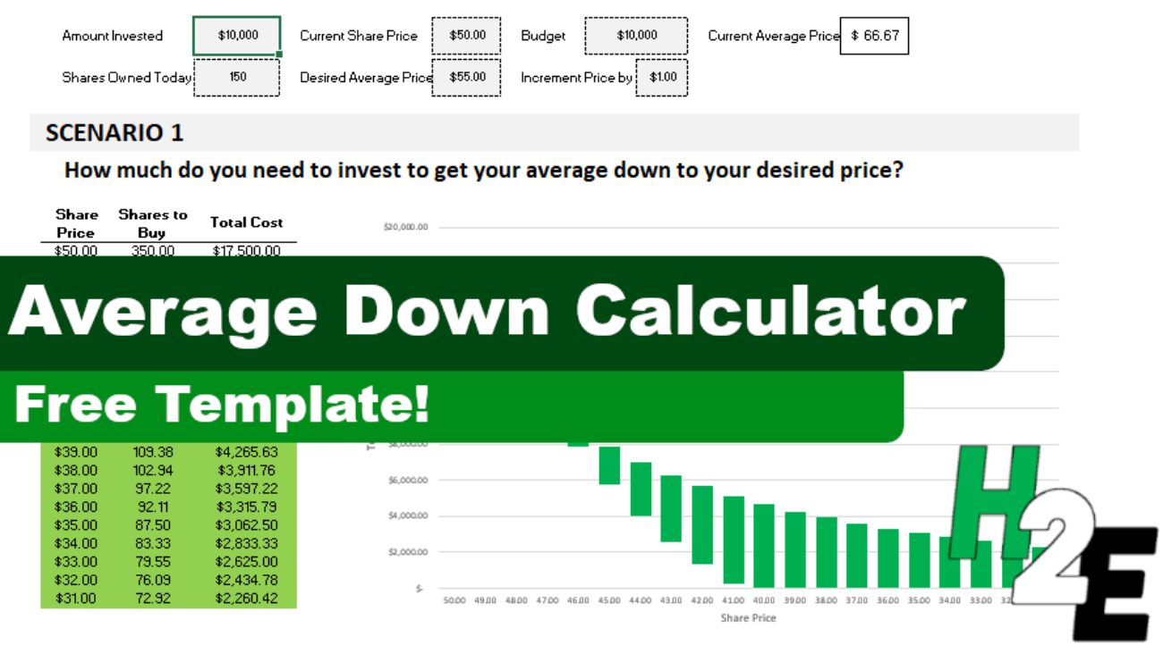
Average down calculator showing how to get down to an average desired price.

If all the data points aren’t filled in or it looks like the chart doesn’t go all the way to the right, this is a sign you need to fix your Increment Price by value. Enter a smaller price increment and you’ll see more data points and a more complete chart.

2. How low you can get your average

The second scenario ignores the desired average price and simply tells you the different average prices you can average down to if you buy at the current price. This is good if you don’t have a specific average in mind and just want to see how low you might be able to go.

Average down calculator showing how low you can get your average.

You’ll notice on the x-axis it refers to the average price rather than the share price in the earlier chart.

Please note that the template is locked down and this is to prevent overwriting formulas which could lead to errors in the calculations and the charts.

Download the file

You can download the file for free, from here. The free version is limited to five price points. On the full version, there are 20 different prices, no ads, and the file is unlocked.


If you liked this Average Down Calculator Template, please give this site a like on Facebook and also be sure to check out some of the many templates that we have available for download. You can also follow us on Twitter and YouTube.