Wildcards in Excel are special characters that can stand in for other characters in a text string. They are incredibly useful for finding, filtering, or matching data when you only have a partial match. Think of them as “jokers” you can use in your formulas.
Excel has three wildcard characters, and they only work with text, not numbers.
The 3 Excel Wildcards
- Asterisk (
*)- What it does: Represents any number of characters, including zero characters.
- Example:
"Sm*"would match “Smith”, “Smythe”, or even just “Sm”. - Example:
"*sales*"would match “Total Sales”, “Sales-Q1”, or “Sales”.
- Question Mark (
?)- What it does: Represents exactly one character in a specific position.
- Example:
"Sm?th"would match “Smith” and “Smyth” but not “Smythe”. - Example:
"??-100"would match “US-100”, “CA-100”, and “MX-100” but not “USA-100”.
- Tilde (
~)- What it does: This is the “escape” character. It tells Excel to treat the next character as a normal character, not a wildcard. You use this when you are actually searching for a literal asterisk or question mark.
- Example:
"FY25~*"would find the exact text “FY25*” (and would not treat the*as a wildcard). - Example:
"What~?"would find the exact text “What?”
How to Use Wildcards in Excel Functions
Wildcards don’t work in all Excel functions, but they work in many of the most popular ones, including COUNTIF, SUMIF, AVERAGEIF, VLOOKUP, HLOOKUP, XLOOKUP, MATCH, and SEARCH.
Important: When using wildcards in a function, the criteria (the part with the wildcard) must always be enclosed in double quotation marks (" ").
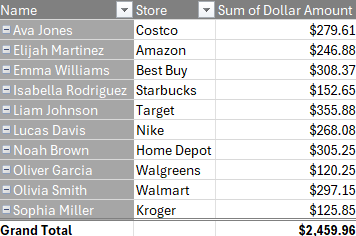
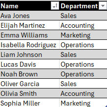
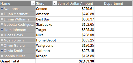
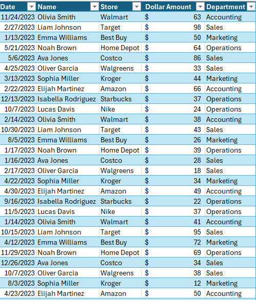
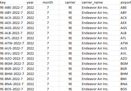
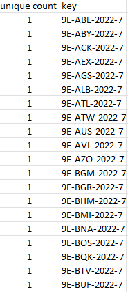
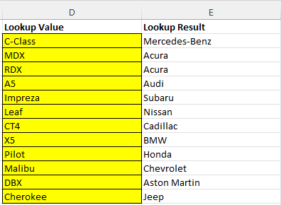
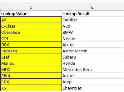
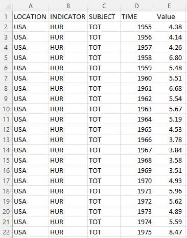
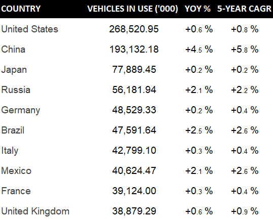
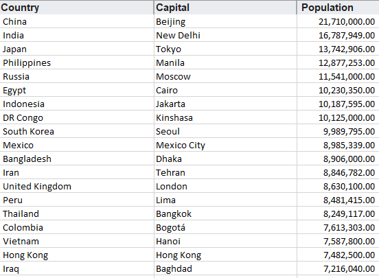
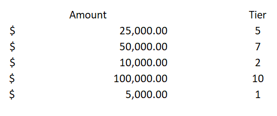
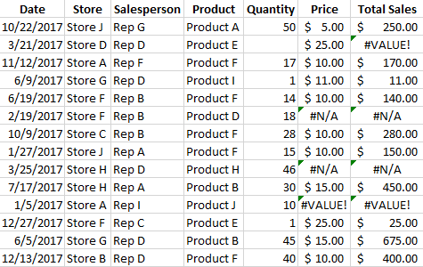
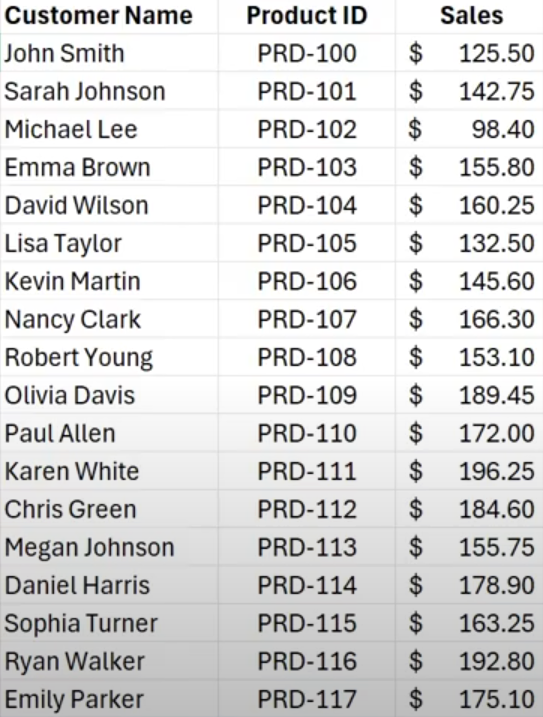
Let’s go over an example using the data set below, which shows customer name, product ID, and sales.
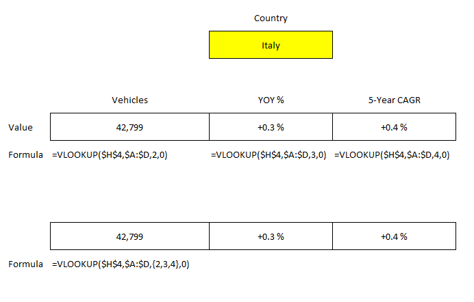
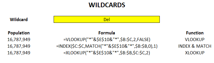
Using VLOOKUP with wildcards
I can use the VLOOKUP function to find a value that Starts with ‘John S’ and this can be done by adding a wildcard afterwards. With my table in columns A:C, this is how I setup my formula:
=VLOOKUP("John S*",A:C,3,false)
This returns a value of $125.50, which is the first customer in the list, John Smith.
Let’s suppose I don’t want to hardcode my search values. Instead, let’s link to a cell and add the asterisk afterwards. In the below example, I have the lookup value showing in cell F2.
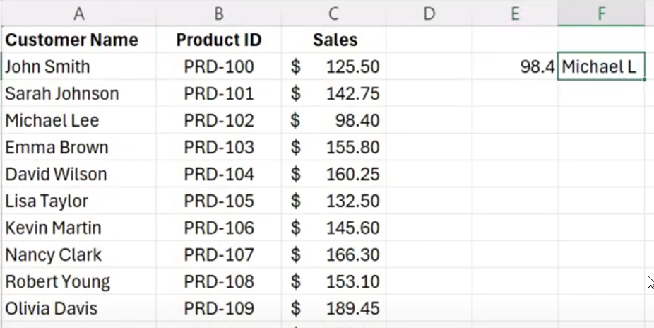
If I want to look up any value that starts with Michael L, I would setup my formulas as follows:
=VLOOKUP(F2&"*",A:C,3,false)
The key here is to use the & to connect the lookup value with the wildcard, and this is the same as manually hardcoding the lookup value with the wildcard. But by linking it to a specific cell, it can make your search criteria more dynamic. You can just change the cell in F2 without changing anything else in your formula.
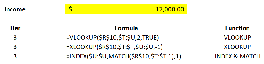
Using XLOOKUP with wildcards
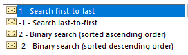
XLOOKUP works in a similar way to VLOOKUP but there are a couple of key differences to consider. The first is that the order of the arguments is different. The other is that by default, wildcards are not enabled. You need to specify in the second-last argument (search mode), that you want to use wildcards. That argument needs to be set to a value of 2. Here is how you would setup the same wildcard lookup with XLOOKUP:
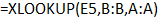
=XLOOKUP(F2&"*",A:A,C:C,,2)
This produces the same result as in the previous VLOOKUP formula.
Using wildcards to sum up partial matches
Another way you can use wildcards is to sum or average values when a criteria is met. In the example above, I’m going to sum all the amounts where the name contains “Johnson” somewhere in the text. Here’s how that would work within a SUMIF function:
=SUMIF(A:A,"*Johnson*",C:C)
This formula uses two asterisks, one before and one after Johnson. As long as it is somewhere within the text, it will be summed up. The formula returns a value of $419.25, the total of all the values that contain Johnson.
In some cases, you may not want to use the asterisk but instead use a wildcard for just a single character. This is when you might use the ? symbol. In the following example, I’m going to sum up all the product IDs that start with PRD-11, but I am only searching for one additional character:
=SUMIF(B:B,”PRD-11?”,C:C)
This adds up to 1,748.60. It will sum up all product IDs between PRD-110 through to PRD-119. But if I had a product ID that went a character longer, such as PRD-1100, that would not be included since that would be more than one additional character. With the ? wildcard, it specifies how many additional characters I am looking for. Each ? represents one character. This is a more specific wildcard search than simply using the asterisk.
If you liked this post on How to Use Wildcards in Excel, please give this site a like on Facebook and also be sure to check out some of the many templates that we have available for download. You can also follow me on Twitter and YouTube. Also, please consider buying me a coffee if you find my website helpful and would like to support it.