

If you’re looking up data, often times just using a VLOOKUP function can be enough to get you your desired result. Sometimes, however, it doesn’t do enough, especially if you’re looking for a partial match.
While you can set VLOOKUP to pull an approximate match rather than an exact match, that may not provide you with the desired results, especially if you’re using text.
Consider the following situation where you’ve got a series of charges from your credit card statement and want to find a particular vendor:
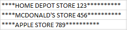
In the above example, let’s assume I’m looking for McDonald’s and do a regular VLOOKUP and set the approximate match argument to true, my formula looks like this:
=VLOOKUP(“MCDONALD’S”,B:B,1,TRUE)
And the result I get is this
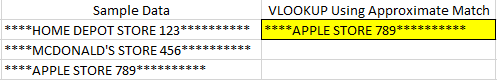
As you can see, it’s not what I was hoping for. Excel can’t figure out that I’m looking for the second result, and simply gives me the last one.
Using Numbers with the Approximate Match
The approximate match isn’t useless in VLOOKUP, in fact, when it comes to numbers, it can be very accurate.
Consider the following example:
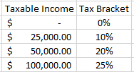
If I want to find out the tax bracket that a given income level relates to, I’ll use this formula
=VLOOKUP(G11,D:E,2,TRUE)
Assume column D is the taxable income and column E is the tax bracket %, with the taxable income I input being in cell G11.
Using this formula, if I put an income of $0 in G11, my tax bracket is correctly returned as 0%. It’s not until I enter $25,000 that it will return 10%.
Excel understands numbers better than words, and so it knows that since $24,999 is not greater than or equal to $25,000, that it still belongs in the first tax bracket, the one that was 0% and started at $0.
If I enter $105,000 as my income amount, then it also correctly knows that I’m in the 25% tax bracket since that is the highest bracket in the list.
If, however, I don’t put the brackets in the correct order my results won’t be the same. In order for this type of calculation to work, you need to start from the lowest value to the highest.
How Can We Get Text to Work?
If you want your partial text matches to work, you’ll want to use wildcards. What you can do is add an asterisk before and after your search term, which will then return even a partial match. Here’s an example of how the updated formula might look from the first example:
=VLOOKUP(“*MCDONALD’S*”,B:B,1,FALSE)
This might look a bit confusing since now I’m actually not looking for an approximate match, but rather an exact one, as indicated by the FALSE argument at the end.
But because the asterisks will grab everything before and after my text, technically I do want it to match exactly, since it’ll search for my string as well as anything before and after it.
The result:
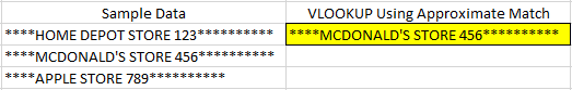
*Note that the formula is not case sensitive. Whether I type in MCDONALD’S or mcdonald’s, it would have no impact on my result.
As you can see, now I get the partial match that I was looking for. The danger, however, is that your partial string isn’t unique enough. If I were to use the word STORE as my string, I would get the first result that is a match, and in this case that would not be what I want.
Because VLOOKUP will return the value for the first time there was a result, you want to ensure its not a common string that will be found more than once.


