How to Use VLOOKUP With Multiple Sheets

VLOOKUP is a popular function in Excel because of how powerful and easy it is to use. You can even use it to look up values on different sheets. And in this post, I’ll show you how you can do so dynamically so that you don’t always need to be adjusting your formula.

Why you might want to use multiple sheets in the first place

There are good reasons to use multiple sheets in your workbook. The first is that it makes it easier to organize your data. The second is that it can make your formulas more efficient. For example, running calculations on a tab where you have tens of thousands of rows would not be optimal and if you can split that up into smaller worksheets, you can make your formulas smaller in scope.

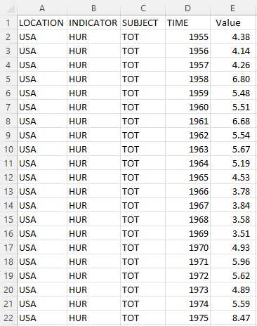
In my example, I’ve downloaded historical unemployment numbers by country. And rather than putting that data all into one sheet, I’ve created multiple tabs for countries. Not all of them, but just a few that I want to do lookups on:

Each tab is named after the country abbreviation in the data to make it easy to know what’s in each sheet. And inside each sheet is data that is formatted in the same way:

Creating the formula

If I just wanted to lookup the value for the United States’ unemployment rate from 1955, my formula would look as follows:

=VLOOKUP(1955,USA!D:E,2,FALSE)

I could replace 1955 with a cell reference. But other than that, this is in essence what the formula in its simplest form would look like. I’m looking up the USA tab as indicated by the ! symbol that comes after the sheet name. You don’t actually need to enter the ! mark. You can just type in the formula and then when you get to the lookup range, jump over to that tab and select your range — Excel will automatically add the exclamation mark for you.

While this formula works, it isn’t versatile. If I wanted to look up a different tab, I would need to change the reference, since it is hardcoded.

Making the formula dynamic

I have created named ranges for the country and year values:

What I want to be able to do is change any one of them and for my lookup formula to extract the correct value. The key to making this work is by including the INDIRECT function. With that, I can reference the specific range I need and use a dynamic tab name. Inside the INDIRECT function, I can concatenate the country value with the range:

INDIRECT(Country&”!D:E”)

But this on its own only specifies a range. I need to include it in the lookup formula for it to work:

=VLOOKUP(Year,INDIRECT(Country&”!D:E”),2,FALSE)

‘Year’ and ‘Country’ are the named ranges that I have used above. The key thing to remember is the exclamation mark that comes afterward and the range. By doing this, now I can change my formula to automatically pull from the correct tab while also looking up the year. It avoids me having to change the formula manually every time I want to use different tabs. It returns the same value as if I were to enter it myself:

If you liked this post on How to Use VLOOKUP With Multiple Sheets, please give this site a like on Facebook and also be sure to check out some of the many templates that we have available for download. You can also follow us on Twitter and YouTube.