H2Ecalcstreaks

How to Calculate Streaks in Excel

Do you want to calculate how long a team’s winning streak is, or how many cells in a row meet certain criteria? In this post, I’ll show you how you can calculate streaks in Excel. Unlike a simple count function, this will require being able to reset your count and go back to zero. I’ll show how this can be done using an easy approach that involves a helper column, and a more challenging way that doesn’t require one.

The easy way to calculate streaks

Here are some results, showing wins (W), losses (L), and ties (T).

Game results on a spreadsheet showing wins, losses, and ties.

The helper column I’m going to create will evaluate the criteria. And the criteria, in this case, will be whether the result is a win. For this, all that’s required is a simple IF statement checking if the value is a W:

=IF(A2="W",1,0)

If the result is a W, the formula will return a value of 1, otherwise, it will be 0:
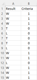
Criteria column showing a 1 value for W and 0 for L.

Next to that column, I will create another one for the actual streak. This formula will look at the criteria column, and if it equals 0, then the streak is 0. If it’s a value of 1, then it will add on to the previous value in the streak column, and thus, add on to it. The formula is as follows:

=IF(B2=0,0,B2+C3)

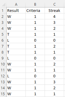
And that results in the following calculations:
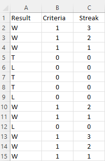
Result, Criteria, and Streak columns for calculating streaks in Excel.

The assumption here is that the earlier results are at the bottom and the most recent games are at the top.

If you wanted to calculate how many games were either won or tied in a row, and thus, an undefeated streak, all you need to do here is to adjust the criteria column. The updated formula would be this:

=IF(OR(A2="W",A2="T"),1,0)

And now the streak values change:

Calculating an undefeated streak in Excel with a helper column.

The difficult approach, without helper columns

If you don’t want to use a helper column, calculating streaks is a bit more challenging. You will be using an IF function and checking for criteria, but this time you’ll need to always adjust your starting point (i.e where the streak is 0). And that will need to be within a SUM function to ensure that the values are added. The key to making this work is using the INDIRECT function so that you have control over the exact range you want to include.

Inside that function, I’ll start with column A and use the current row the cell is on, which can be done using the ROW function. Here’s how it starts:

INDIRECT("A"&ROW(B2)&":A"

B2 reflects the first cell in the streak calculation, and it will return a value of 2. The last cell needs to be the last time the streak was broken — when the team recorded a loss. This involves using the MATCH function and searching for an “L”. That formula is as follows:

MATCH("L",INDIRECT("A"&ROW(B2)&":A15"),0)

Here again, I use the ROW function and as my ending cell, I put A15, which is the last cell in the range. This could be adjusted to use a MAX function to make it variable. Since the MATCH function will return a number corresponding to its position within the range (e.g. it won’t return the actual row), I will adjust for the row number immediately above the first cell to be searched. In this case, since I’m searching cells A2:A15, I need to add 1 to ensure I get the row number and adjust for the fact that the MATCH function doesn’t begin from the very first row. I will add all this together into my earlier formula:

INDIRECT("A"&ROW(B2)&":A"&MATCH("L",INDIRECT("A"&ROW(B2)&":A15"),0)+ROW(B1))

Now I have to enclose this within the IF function and check to see if the result is a W:

IF(INDIRECT("A"&ROW(B2)&":A"&MATCH("L",INDIRECT("A"&ROW(B2)&":A15"),0)+ROW(B1))="W",1,0)

Then, I put that all within a SUM function:

SUM(IF(INDIRECT("A"&ROW(B2)&":A"&MATCH("L",INDIRECT("A"&ROW(B2)&":A15"),0)+ROW(B1))="W",1,0))

The one last adjustment that’s necessary is to account for if there is no loss found and the team starts on a winning streak. For this, I’ll add an IFERROR function just before the MATCH function so that if it evaluates to a 0 (after adding the 1), then it will default to the last row (15):

IFERROR(MATCH("L",INDIRECT("A"&ROW(B2)&":A15"),0)+ROW(B1),15)

The full formula for calculating the win streak is the following:

=SUM(IF(INDIRECT("A"&ROW(B2)&":A"&IFERROR(MATCH("L",INDIRECT("A"&ROW(B2)&":A15"),0)+ROW(B1),15))="W",1,0))

Given how complex this formula is, it can get messy if you create too many conditions in it. And if you do have multiple criteria you’re dealing with, then the first approach may be the more practical one to use in that case.


If you liked this post on How to Calculate Streaks in Excel, please give this site a like on Facebook and also be sure to check out some of the many templates that we have available for download. You can also follow us on Twitter and YouTube.

H2Evlookupmultiple1

How to Use VLOOKUP With Multiple Sheets

VLOOKUP is a popular function in Excel because of how powerful and easy it is to use. You can even use it to look up values on different sheets. And in this post, I’ll show you how you can do so dynamically so that you don’t always need to be adjusting your formula.

Why you might want to use multiple sheets in the first place

There are good reasons to use multiple sheets in your workbook. The first is that it makes it easier to organize your data. The second is that it can make your formulas more efficient. For example, running calculations on a tab where you have tens of thousands of rows would not be optimal and if you can split that up into smaller worksheets, you can make your formulas smaller in scope.

In my example, I’ve downloaded historical unemployment numbers by country. And rather than putting that data all into one sheet, I’ve created multiple tabs for countries. Not all of them, but just a few that I want to do lookups on:

Multiple tabs created for different countries.

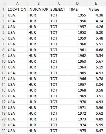
Each tab is named after the country abbreviation in the data to make it easy to know what’s in each sheet. And inside each sheet is data that is formatted in the same way:

Historical unemployment data for the United States.

Creating the formula

If I just wanted to lookup the value for the United States’ unemployment rate from 1955, my formula would look as follows:

=VLOOKUP(1955,USA!D:E,2,FALSE)

I could replace 1955 with a cell reference. But other than that, this is in essence what the formula in its simplest form would look like. I’m looking up the USA tab as indicated by the ! symbol that comes after the sheet name. You don’t actually need to enter the ! mark. You can just type in the formula and then when you get to the lookup range, jump over to that tab and select your range — Excel will automatically add the exclamation mark for you.

While this formula works, it isn’t versatile. If I wanted to look up a different tab, I would need to change the reference, since it is hardcoded.

Making the formula dynamic

I have created named ranges for the country and year values:

What I want to be able to do is change any one of them and for my lookup formula to extract the correct value. The key to making this work is by including the INDIRECT function. With that, I can reference the specific range I need and use a dynamic tab name. Inside the INDIRECT function, I can concatenate the country value with the range:

INDIRECT(Country&”!D:E”)

But this on its own only specifies a range. I need to include it in the lookup formula for it to work:

=VLOOKUP(Year,INDIRECT(Country&”!D:E”),2,FALSE)

‘Year’ and ‘Country’ are the named ranges that I have used above. The key thing to remember is the exclamation mark that comes afterward and the range. By doing this, now I can change my formula to automatically pull from the correct tab while also looking up the year. It avoids me having to change the formula manually every time I want to use different tabs. It returns the same value as if I were to enter it myself:


If you liked this post on How to Use VLOOKUP With Multiple Sheets, please give this site a like on Facebook and also be sure to check out some of the many templates that we have available for download. You can also follow us on Twitter and YouTube.

H2ESlowSpreadsheet-min

7 Ways to Fix a Slow Spreadsheet

Is your spreadsheet running slow or constantly freezing and crashing on you? There are many ways you can make it quicker and more efficient. Below, I’ll cover seven different ways you can fix some of the more common reasons your file may not running well.

1. Turn off calculations for the workbook

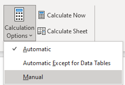
The first thing you can do is to turn off calculations. If you don’t need your data to constantly be updating, then the easiest way to ease the load of your spreadsheet is to make sure those formulas don’t keep calculating. To do this, you can go to the Formulas tab and under the Calculation group, select Calculation Options and choose Manual:

How to select manual calculations in Excel.

You can always turn the formulas back on and use F9 to do a force calculation. But if you don’t want to re-calculate everything, a quick trick you can do is to use Find and Replace and replace the equals sign (“=”) with equals. It seems redundant but doing this will refresh your formulas and recalculate the range you selected. This can be an easier alternative to enabling calculations for everything and then having to wait for every calculation to update.

The danger with turning off calculations is that you could end up looking at data that hasn’t been updated and potentially incorrect values as a result of that. This is why you’ll always want to be careful when turning off calculations for an entire workbook.

2. Turn off calculations for individual worksheets

If you don’t want to turn off everything, you can turn off the calculations for specific worksheets. Although there isn’t a way from the calculation options to specify which sheets to turn off, you can do this through a macro.

To do this, go into visual basic (ALT+F11) and go into the ThisWorkbook object:

VBA Project list.

We’ll want to turn off calculations when the workbook is first opened so you don’t have to remember to do it later. The initial subprocedure looks as follows:


Private Sub Workbook_Open()

End Sub


To turn off a calculation, you just need a single line of code:

Worksheets(“Sheet1”).EnableCalculation = False

Then entire subprocedure look as follows:


Private Sub Workbook_Open()

Worksheets(“Sheet1”).EnableCalculation = False

End Sub


Where Sheet1 is the name of the sheet that you want to turn calculations off for. And if you want to turn them back on, you change the value from False to True.

This isn’t the easiest option, especially if you aren’t familiar with macros or don’t want to worry about coding anything. But with VBA you can turn off the calculations and then use a button to turn them back on.

3. Separate the data into multiple tabs

If you have a data set that includes multiple years worth of data, you may want to consider breaking it up. Have one tab for the current year, one for the previous year, and so on.

Using the INDIRECT function, you can refer to different worksheets in your file. By naming a header the same name as a tab (e.g. ‘2020’), you can make your formulas dynamic and pointing to a different worksheet as opposed to one very large tab. Looking up 10,000 rows in one tab versus 50,000 rows in a massive collection of all your data can significantly improve the time it takes for your calculations to run.

4. Separate data into multiple files

A more drastic move than breaking up data into different tabs is moving them onto completely different files. If you’re carrying lots of old data into one big spreadsheet, consider archiving some of it and saving it in another file. Unless you really need access to the old data all the time, it might make a lot of sense to break up your files and to keep your current version as lean as possible. You could even have your data on one file and a separate file for your reporting while using PowerQuery to create a snapshot of your data and simply refreshing it as you need it.

5. Use COUNTA and INDIRECT to limit the scope of your calculations

The INDIRECT function can also help you to ensure your formulas don’t include too many rows or columns. If you select an entire column to run your calculations on rather than just the first couple hundred rows that actually have data in them is another way you can slow down your spreadsheet.

To do this, you can use the COUNTA function on a range to determine how many cells have values in them. The formula is a simple one that you can run on an entire column:

=COUNTA(“A:A”)

Then, using the INDIRECT function, you can write a formula that does something like this:

=SUM(INDIRECT(“A1:A”&B1))

B1 in the example above contains the COUNTA formula and will give you the total number of rows that are used. Rather than doing this:

=SUM(A:A)

and selecting everything in column A to sum up, you can shrink your range down using a combination of the INDIRECT and the COUNTA function. This can be a time-saver when you’re dealing with complex calculations, especially if there are thousands of rows of data.

6. Minimize formulas and utilize pivot tables where possible

Another way to cut down on resources is to make use of pivot tables. Pivot Tables are more efficient than formulas and using them can help make your spreadsheet run smoother. The one drawback is that they’re not as flexible as formulas are. Refreshing the data also takes seconds and you don’t have to worry about turning calculations off.

7. Make sure your worksheets aren’t too big

Large files can take long to open and they freeze up a lot. A common problem I see is that worksheets are sometimes thousands of rows long even though there’s nothing there. This can happen if you download a large data set into a sheet and clear it out later. And although those rows may no longer be occupied with data, they’re still technically taking up space. This can add several MB onto a file and make it a lot more difficult to run.

How can you spot this issue? An easy way is to cycle through the tabs and click CTRL+END. You’ll be taken to the last cell in your sheet. If that takes you far beyond your last row or column of data, then that tells you your sheet is using up more data than it needs to. What you can do is delete all the cells in between the last cell (using CTRL+END) and the last cell that actually contains information in it. Then, save the file. You should see your file come down in size. Do this for each worksheet that has this issue. Even though the cells appear to be empty, they can be making your file unnecessarily large.


If you liked this post on 7 ways to fix a slow spreadsheet please give this site a like on Facebook and also be sure to check out some of the many templates that we have available for download. You can also follow us on Twitter and YouTube.

multipledropdowns

How to Create a Drop Down List in Excel

If you need to collect user input in an Excel spreadsheet, you’ll want to be able to minimize errors and typos in the information that you receive. That’s why it’s important to know how to create a drop-down list in Excel as it will limit the selections that someone will have to choose from. Using lists can prevent someone from making a data-entry error which can save you a lot of grief later on when you go to analyze the data. Here are the steps involved in creating a drop-down list:

1. Create the list of items that you want your user(s) to be able to select from

The first step in learning how to create a drop-down list in Excel is to first identify your list of selections. This seems like an obvious step but sometimes people don’t actually set aside a space on their spreadsheet for a list of items and simply hardcode the selections later on. By listing the items, you can easily modify them later and visually see what are the user’s options. In this example, I’m going to give a user a list of stores to choose from:

List of stores for a drop-down list in Excel.

2. Convert the list into a table

You don’t need to do this but there’s an important reason to do so: if you add items later, the range you select for your drop-down list will automatically update. If you just select a regular range, you’ll have to modify it if you add more options to it later. The goal is to make this as easy as possible. And if you always have to adjust the range for subsequent additions, it’s an easy step to miss.

To create a table, just select your range and on the Insert tab, click on the Table button:

Creating a table in Excel.

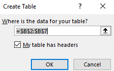
Make sure to include your header in the select and that you tick off that your data includes headers:

Create table and specify that it includes headers to ensure your drop-down list contains the correct selections.

Now you’ll likely see some automatic formatting applied to your list that shows it’s now a table:

Table created in Excel that can now be used for a drop-down list.

3. Create a named range

Within the table, where you selections are, create a named range. Just select the cells you want to use (they should be everything in the column) and just assign a name to them. Here’s how you can create named ranges in Excel. Don’t worry if after assigning a named range it doesn’t reflect the name in the reference in the Name Box. Since it’s a table, it’ll still reference the table name. In my example, I created a named range called Stores.

By referencing named ranges, you avoid having to rely on cell references and it’ll make your list dynamic. This is also going to play an important role if you want to have multiple lists, with one based on a prior list’s selections.

4. Create the drop-down list using data validation

Decide where you want your drop-down list will go. Sometimes it’s helpful to highlight it so that it’s easy to distinguish it from other cells. In my example, I’ve highlighted the cell in yellow. Then, click on Data Validation under the Data tab:

Select data validation to create your drop-down list in Excel.

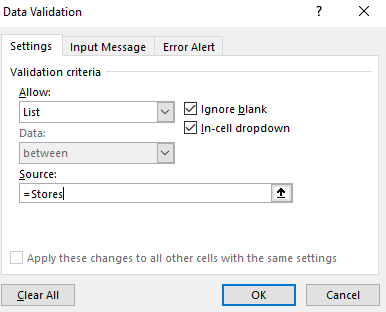
From there, select a List for your range. The list should be equal to your named range or the range of cells you want to use for your drop-down selections. I’m going to set this equal to the Stores named range. When using named ranges, always put the equals sign in front:

Setting your named range to a named range. This will make it easy for managing your drop-down list.

Now, the drop-down list is ready to go:

A drop-down list in action.

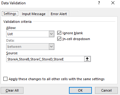
You don’t have to use a named range for a list. You can just select the range manually or you can just type the options in:

Manually entering in selections in a drop-down list.

As you can imagine, this is a very cumbersome approach and can be very time consuming if you have a long list. Unless you’ve got only a few options that will never change (e.g. yes/no), it probably doesn’t make sense to manually enter the selections this way.

A key benefit of using a named range, within a table, is that if you add selections they’re automatically updated. I’m going to add StoreF to my list of stores. And all that involves is just typing that store directly below the last value in the table:

Adding another store to the table is very easy to do and it will automatically update your drop-down list.

If I go back to my drop-down list, the selection’s already there:

A drop-down list is now updated.

Had I manually entered the drop-down selections, the list wouldn’t update automatically. I would need to adjust it manually. This can obviously save a lot of time if your list will grow over time.

Creating drop-down lists based on prior drop-down list selections

If you’ve got multiple drop-down lists and want to make them dependent on prior selections, this section is for you. The good news is that it’s largely the same approach. If you know how to create a drop-down list in Excel, adding dependent lists won’t be much more difficult.

You can make some very complicated and nested drop-down lists possible by using a combination of tables and named ranges. In my example, suppose not every store sells the same product. So a scenario can be that a customer is placing an order and selects a store and then in their next selection they can select from a product that’s available in that specific store.

What we’ll need to do in that case is create another named range for that specific store. That range will show the products that store has available. Now, unless the number of selections will remain the same (e.g. same number of stores as there are products available in that store) — which I’m going to guess is unlikely — you’ll want to create a separate table. In this example, I’ll create a list of products just for StoreA, and convert it into a table:

A drop-down for a list of products sold at StoreA.

I also need to select the list of products and assign a named range to them. For the named range, it’s important that I assign it the name of the store: StoreA. The reason this is important is that this becomes key to my formula in order to link the previous drop-down selection (where I chose a store) to the new named range.

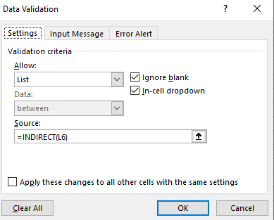
In the next data validation list, I’ll need to use the INDIRECT function and refer to the previous selection (for stores). In my spreadsheet, the cell that contained the store selection was L6, and so my INDIRECT function will need to reference that in the data validation:

Using an indirect formula to reference a prior drop-down list selection.

Since the range is hardcoded in the data validation settings, if you move your drop-down box you’ll need to update the indirect formulas. Here’s how my second drop-down selection looks now:

Multiple drop-down lists.

By using the INDIRECT function, the drop-down selections for the product category were updated based on the StoreA selection. I’ll create another table for StoreB where only ProductD and ProductE will be available. Now, when I go to select StoreB, these are what my selections look like:

Drop-down list selections based on a different store.

The named range is set to StoreB for those selections. What we can do is drill down even further. Suppose ProductA and ProductB came in various sizes – for simplicity’s sake, I’ll just call them Size1, Size2, and Size3. To do that, I’ll again need to create a table for those selections, and a named range that refers to the product name:

Another list for size options based on product selections.

These ranges are called ProductA and ProductB. I’ve put them in separate tables because since there are a different number of options, I don’t want them to be part of the same table. If they were in one table then ProductB would include blanks. And if only selected the first two selections then it wouldn’t automatically update if I added more selections.

Here’s what my new drop-down selection now looks like if I select ProductA:

Three drop-down lists to select options from.

For the third drop-down selection, I have to again use data validation and use the INDIRECT function and refer to the adjacent cell. If I select ProductB, I only have two sizes to choose from. Here’s how the drop-down lists look in action:


If you liked this post on how to create a drop-down list in Excel, please give this site a like on Facebook and also be sure to check out some of the many templates that we have available for download. You can also follow us on Twitter and YouTube.
Referencing Cells in Other Worksheets and Workbooks using the INDIRECT function

When working with multiple worksheets or tabs, it becomes useful to reference them in formulas or to consolidate data. First, I’ll look at working with different tabs.
Referencing Other Tabs

The easiest way to refer to a cell in another tab is to start a formula with the = sign, and then click over to the other tab and click on the cell you want to reference.  In the following example I am typing a formula in tab A but will reference cell B6 on tab B.
Note the reference in the formula bar:
=B!B6
The tab is denoted by the ! after the tab name. If I wanted to reference tab A it would look as follows:
=A!B6
But what if my tab wasn’t all one word, and the tab was named A and B? In this case, I would need to use apostrophes:
=’A and B’!B6
So to summarize, the naming convention for referencing another sheet is:
SHEET1!A1 or ’SHEET 1’!A1


Linking to other Spreadsheets

Now let’s assume the cell you want to reference isn’t in this same workbook, then the reference looks a bit different. If the workbook is open:
=[Workbookname] SHEET1!A1

The key difference is you are adding the workbookname. This method will work if the workbook is open, but not recommended if you are referencing a workbook that is closed because Excel might not know which workbook you want to reference and cause errors. To properly reference a closed workbook, use the following:
=’C:Desktop[Workbookname.xlsx]SHEET1!A1
The above formula will work if the workbook is saved on my desktop.
In this example I only used a single cell, but you can just as easily reference a range. Change A1 to A1:A10 and you are referencing a range instead of a cell. This comes in useful if you want to use the reference in a lookup.
Using the INDIRECTFunction

Referencing other worksheets and tabs is not difficult once you get used to the syntax, but if you had dozens of tabs or workbooks you wanted to reference, it might get tiresome to keep doing this. That’s where the INDIRECT function comes in handy. You can use formulas to populate these cell references so that you don’t have to re-type them or even use find and replace.
Imagine you have sales data on multiple tabs. Each tab represents a year. So if I want to summarize data from five different years (tabs), that’s five different references I have to use. Or I can use the INDIRECT function. The way the formula works is you can enter the entire location of the cell that you want to reference. The benefit is being able to use relative and absolute references in place of having to type out the full address over and over again.
Here is a comparison of how the references would look using each method:
In the indirect function, I am able to use a relative reference for the year. If I enter the formula in cell B4, all I have to do is copy the formula down and it will reference all the other years(tabs) without having to re-type the full location. The benefit here is apparent when you are dealing with many different tabs. In column C I am unable to do this and have to re-key each cell individually.
The tricky part of using the indirect function is making sure you are correctly combining the ampersands, variables, and constants. The ampersand you use to join a constant and a variable within the INDIRECT formula. In this example, the variable is the year (tab name). The constant is the syntax (!) and the cell reference (A1), since their values will never change.  Never put the variable in quotations, only constants. 
Here is a breakdown of the logic of the formula in cell B4:
Because I am referencing another tab (not another workbook), I need to start with the worksheet name. Since I have a variable for the worksheet name, I start with the reference to cell A4, which contains the name of my worksheet: 
=INDIRECT(A4
The remainder of the formula is going to be !A1, or, the constants. To add the constants, I need to add the ampersand, open quotations, enter the constants, and close the quotations and the formula:
=INDIRECT(A4&”!A1”)
You can alternate between constant and variable as much as you like but they have to be linked by an ampersand. You also don’t need to begin the INDIRECT function with a variable, it can be a constant.
Using INDIRECT with Workbooks
You can use the INDIRECT function to reference other workbooks, but unfortunately a limitation of the formula is that it is unable to get data from a closed workbook. So unless you plan to have the workbooks open, the formula will not be of much help here. The formula is most helpful when dealing with multiple tabs in a single workbook.
Avoiding Errors

Some key things to remember when referencing other sheets or workbooks:
  • Syntax is important, like in all formulas, but in these cases it’s very easy to make an error. Remember the !  comes right before the cell reference, and in the case of other workbooks, ‘! precedes it.
  • The INDIRECT function will help expedite referencing other tabs, but cannot help you with referencing closed workbooks.
  • If your tabs do not follow a consistent, predictable pattern then a formula won’t be able to help you much
  • You won’t be able to get data from closed workbooks that are password protected
  • Don’t forget the extension. In my example it was .xlsx but it may be different depending on your version and type of file.