How to Create a Drop Down List in Excel

If you need to collect user input in an Excel spreadsheet, you’ll want to be able to minimize errors and typos in the information that you receive. That’s why it’s important to know how to create a drop-down list in Excel as it will limit the selections that someone will have to choose from. Using lists can prevent someone from making a data-entry error which can save you a lot of grief later on when you go to analyze the data. Here are the steps involved in creating a drop-down list:

1. Create the list of items that you want your user(s) to be able to select from

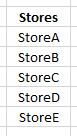
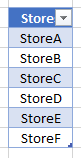
The first step in learning how to create a drop-down list in Excel is to first identify your list of selections. This seems like an obvious step but sometimes people don’t actually set aside a space on their spreadsheet for a list of items and simply hardcode the selections later on. By listing the items, you can easily modify them later and visually see what are the user’s options. In this example, I’m going to give a user a list of stores to choose from:

2. Convert the list into a table

You don’t need to do this but there’s an important reason to do so: if you add items later, the range you select for your drop-down list will automatically update. If you just select a regular range, you’ll have to modify it if you add more options to it later. The goal is to make this as easy as possible. And if you always have to adjust the range for subsequent additions, it’s an easy step to miss.

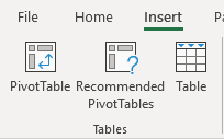
To create a table, just select your range and on the Insert tab, click on the Table button:

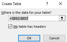
Make sure to include your header in the select and that you tick off that your data includes headers:

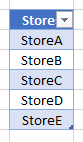
Now you’ll likely see some automatic formatting applied to your list that shows it’s now a table:

3. Create a named range

Within the table, where you selections are, create a named range. Just select the cells you want to use (they should be everything in the column) and just assign a name to them. Here’s how you can create named ranges in Excel. Don’t worry if after assigning a named range it doesn’t reflect the name in the reference in the Name Box. Since it’s a table, it’ll still reference the table name. In my example, I created a named range called Stores.

By referencing named ranges, you avoid having to rely on cell references and it’ll make your list dynamic. This is also going to play an important role if you want to have multiple lists, with one based on a prior list’s selections.

4. Create the drop-down list using data validation

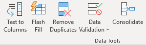
Decide where you want your drop-down list will go. Sometimes it’s helpful to highlight it so that it’s easy to distinguish it from other cells. In my example, I’ve highlighted the cell in yellow. Then, click on Data Validation under the Data tab:

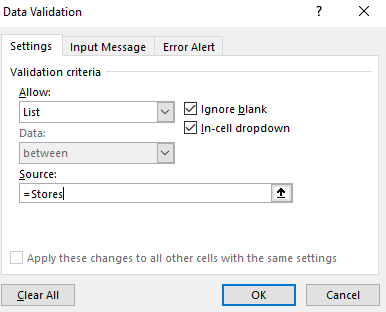
From there, select a List for your range. The list should be equal to your named range or the range of cells you want to use for your drop-down selections. I’m going to set this equal to the Stores named range. When using named ranges, always put the equals sign in front:

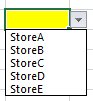
Now, the drop-down list is ready to go:

You don’t have to use a named range for a list. You can just select the range manually or you can just type the options in:

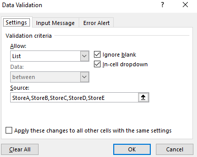
As you can imagine, this is a very cumbersome approach and can be very time consuming if you have a long list. Unless you’ve got only a few options that will never change (e.g. yes/no), it probably doesn’t make sense to manually enter the selections this way.

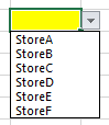
A key benefit of using a named range, within a table, is that if you add selections they’re automatically updated. I’m going to add StoreF to my list of stores. And all that involves is just typing that store directly below the last value in the table:

If I go back to my drop-down list, the selection’s already there:

Had I manually entered the drop-down selections, the list wouldn’t update automatically. I would need to adjust it manually. This can obviously save a lot of time if your list will grow over time.

Creating drop-down lists based on prior drop-down list selections

If you’ve got multiple drop-down lists and want to make them dependent on prior selections, this section is for you. The good news is that it’s largely the same approach. If you know how to create a drop-down list in Excel, adding dependent lists won’t be much more difficult.

You can make some very complicated and nested drop-down lists possible by using a combination of tables and named ranges. In my example, suppose not every store sells the same product. So a scenario can be that a customer is placing an order and selects a store and then in their next selection they can select from a product that’s available in that specific store.

What we’ll need to do in that case is create another named range for that specific store. That range will show the products that store has available. Now, unless the number of selections will remain the same (e.g. same number of stores as there are products available in that store) — which I’m going to guess is unlikely — you’ll want to create a separate table. In this example, I’ll create a list of products just for StoreA, and convert it into a table:

I also need to select the list of products and assign a named range to them. For the named range, it’s important that I assign it the name of the store: StoreA. The reason this is important is that this becomes key to my formula in order to link the previous drop-down selection (where I chose a store) to the new named range.

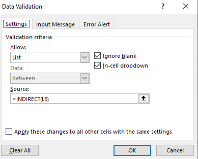
In the next data validation list, I’ll need to use the INDIRECT function and refer to the previous selection (for stores). In my spreadsheet, the cell that contained the store selection was L6, and so my INDIRECT function will need to reference that in the data validation:

Since the range is hardcoded in the data validation settings, if you move your drop-down box you’ll need to update the indirect formulas. Here’s how my second drop-down selection looks now:

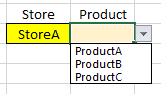
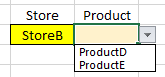
By using the INDIRECT function, the drop-down selections for the product category were updated based on the StoreA selection. I’ll create another table for StoreB where only ProductD and ProductE will be available. Now, when I go to select StoreB, these are what my selections look like:

The named range is set to StoreB for those selections. What we can do is drill down even further. Suppose ProductA and ProductB came in various sizes – for simplicity’s sake, I’ll just call them Size1, Size2, and Size3. To do that, I’ll again need to create a table for those selections, and a named range that refers to the product name:

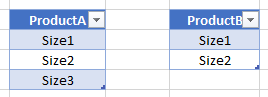
These ranges are called ProductA and ProductB. I’ve put them in separate tables because since there are a different number of options, I don’t want them to be part of the same table. If they were in one table then ProductB would include blanks. And if only selected the first two selections then it wouldn’t automatically update if I added more selections.

Here’s what my new drop-down selection now looks like if I select ProductA:

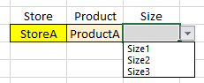
For the third drop-down selection, I have to again use data validation and use the INDIRECT function and refer to the adjacent cell. If I select ProductB, I only have two sizes to choose from. Here’s how the drop-down lists look in action:

If you liked this post on how to create a drop-down list in Excel, please give this site a like on Facebook and also be sure to check out some of the many templates that we have available for download. You can also follow us on Twitter and YouTube.