

Most Excel users likely know how to do a simple VLOOKUP and pull in data where a single field is matched. But what about when you need to match multiple fields? That can be a bit more challenging to pull off and below I’ll show you a couple of ways you can achieve this.
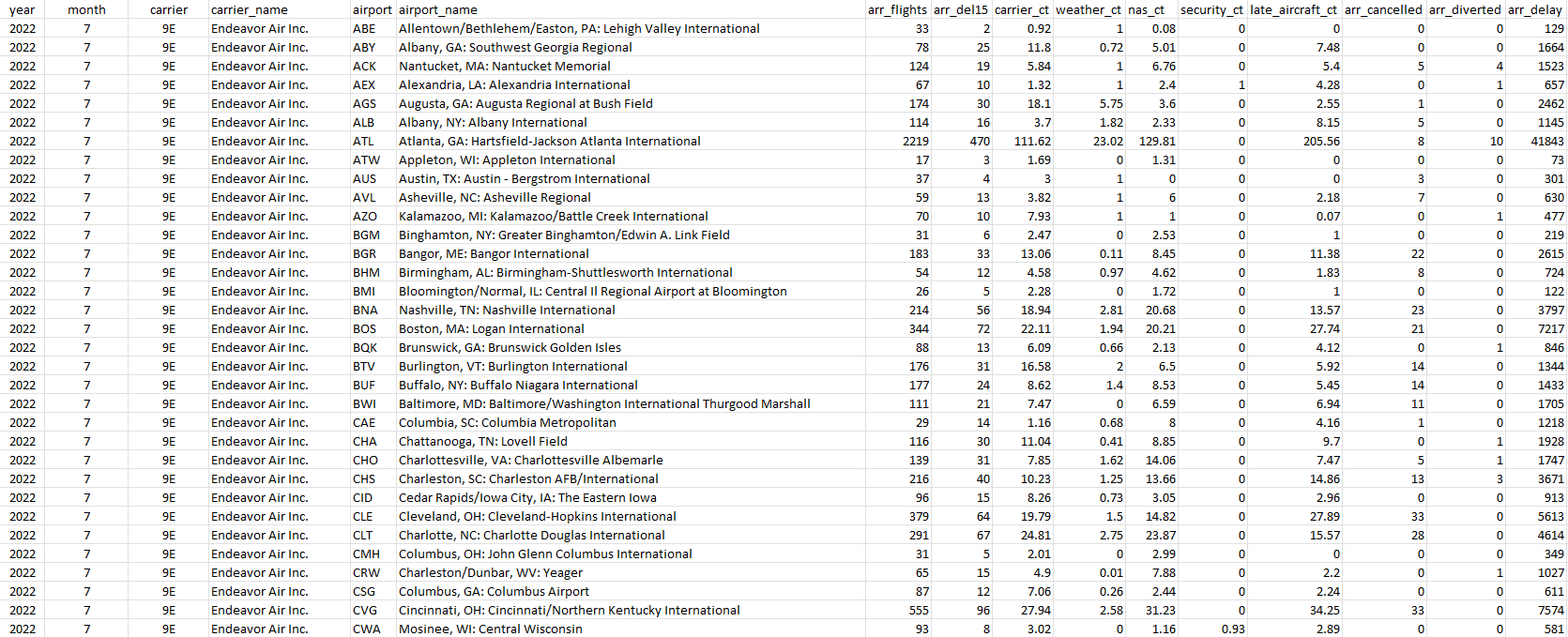
In the following data set, there is information on airports and delay times by specific carriers. Given that there are so many fields here, a simple lookup wouldn’t be helpful here as you need to factor in multiple criteria.
Using a consolidated unique key
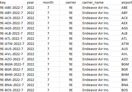
If you are able to create an additional column in your data set, then one option you have available is to create a unique identifier. For example, if I concatenate the carrier code, airport code, month, and year, I can have a key that I could use in a lookup formula. Here’s how that key could look:
The important thing to remember here is that your key should be unique enough so that there is only a single match. For example, if I didn’t include the year and my data includes multiple years, I could potentially have multiple matches for a combination of month, carrier, and airport code.
One way you can test for this is by using the COUNTIF function. This will tell you if there is more than 1 instance of a value. If my key is in column B, here is how that COUNTIF function could look:
=COUNTIF(B2,B:B)If any of the formulas return a value of more than 1, then that will tell you there is a duplicate value:
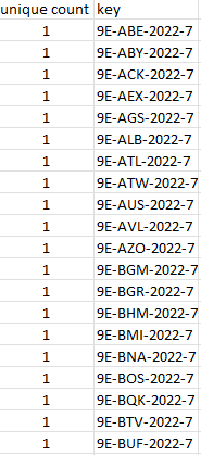
You can use filters to see if there are any values greater than 1 on this list. If there are, then you know you need to adjust your key to add additional criteria so that there are no duplicates. Once you have this accomplished, then you can use this within a VLOOKUP or a combination of INDEX & MATCH. You would just need to use a search criteria that follows the same construct.
Using multiple criteria in a SUMIFS function
Another way you can lookup multiple fields is by using SUMIFS. You can sum the data but you don’t have to. After all, if your criteria is unique, a SUMIFS function would only be summing a single value. And in that sense, it can work similar to a lookup. Using this approach, you don’t have to create any additional columns to make it work.
Here’s how a formula in my data set would look like if I wanted to extract the carrier_delay value for Delta Air Lines (carrier code DL) at the Atlanta airport (airport code ATL), for July 2022:
=SUMIFS(Q:Q,A:A,2022,B:B,7,C:C,"DL",E:E,"ATL")Q is the value I’m extracting, column A relates to the year, column B to the month, column C to the carrier code, and column E to the airport code. Since there is only one corresponding value when filtering for all these combinations, I know my SUMIFS function is only pulling in a single value, and thus, working effectively as a lookup function.
With this approach there is some risk if you don’t first vet your criteria and to check for duplicates. And just to be safe, you’ll probably want to do a check for that before relying on this calculation.
If you like this post on How to Do a Lookup with Multiple Criteria in Excel, please give this site a like on Facebook and also be sure to check out some of the many templates that we have available for download. You can also follow us on Twitter and YouTube.