Using Summation Formulas (SUM, SUMIF(S), SUBTOTAL)

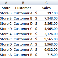
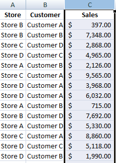
I have saved this sample file here if you would like to look at the data set and have a closer look at how the formulas work.

In this post I will cover some simple summation formulas and when best to use them. I have a sample data set that has stores, customers, and total sales.

Summing Total Sales

If I just wanted to total all the sales then the SUM function would accommodate this easily. There is even a summation button on the Excel ribbon to easily do this.

It is on the right hand side of the Home tab in the Editing group. It will try to determine which cells you want to sum but you can change this range to what you need.

Since my values are in column C my formula would be as follows:

Pretty straightforward, all you need is the column that you want to sum (or specific range if you don’t want everything in the column). This returns the grand total of $256,129 from my data set. Another way I could find out the total is if I just highlight the entire column.

The sum will show in the bottom right corner of my screen in the status bar.

If I right click on any of this area I get the following menu:

If you didn’t see the sum in your status bar this is where you can add it. In my example I could select Minimum and Maximum and then those values would also be calculated for any range that I highlight and show up in the status bar. This makes it easier if you quickly want to see an average, total, min or max by just highlighting a range without having to type a formula each time.

Summing Single Store Sales

But now suppose I just wanted to know the sales of Store A. I could filter the data set, select the column, and see the total in the status bar. But that is a bit tedious to repeat each time if I wanted to see sales by each store. In this case, I could use the SUMIF function.

My formula would look like this:

The first argument, column A, specifies what range I want to look at; the second argument, “Store A”, is what criteria I am looking for; and column C is the final argument, where I want to pull the values from. This formula is saying to look in column A for a value of Store A and add only those related amounts in column C.

Instead of a static reference for Store A I could reference a cell instead, and that would make it easier to apply this formula to multiple stores without having to change the name manually each time.

In the above example assume my store name is in cell E6. If I have the store names going from cell E6:I6 then I could use the following formula:

You will notice I have frozen some of the cells as well. This will allow me to move my formula across without the ranges changing. Below are what my results look like:

Summing Sales by Customer and Store

Now, consider a scenario where I wanted to do a summary of sales by stores and customers. Here I can use the SUMIFS function (only available to Excel 2007 and newer versions). In the formula below I have stores in cells G12:J12 and customers in cells F13:F16:

I can copy this formula and it will be updated based on what store and customer intersect at that point. The summary will look as below:

Unlike with the SUMIF function, the first argument here is the range I want to sum, which is column C. The next argument is the range for my first criteria to look up, column A, followed by the criteria I want to match, which in the first formula is cell E12 (Store A). The next two arguments relate to the next criteria range which is column B for the customers and the customer to be matched which in the formula is cell F13 (Customer A).

With the SUMIFS function you can add more criteria than just two. Simply just add another comma and in the next argument specify the range, followed by the criteria. You can keep adding to it as you need.

How the SUBTOTAL Function Works

Unlike the SUM function, the SUBTOTAL function will perform a calculation based on the filters you have applied (if you have none, it will perform a calculation on all the data in the range). The SUBTOTAL function also has an added argument to tell it what type of calculation it should do:

In the below formula, I am going to total column C again, as I did in the SUM formula initially. However, the additional argument I need in the SUBTOTAL function is defining the calculation. Since I am going to just do a sum, I will set the argument to 9. My formula looks as below:

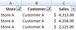
Now, if I were to use filters to show only Store A and Customer A, the SUBTOTAL formula would return the same result as the SUMIFS function did for the intersection of Store A and Customer A.

My formula returns a value of $10,796 with the above filters, which matches the result from the SUMIFS formula. The SUBTOTAL function is useful when you are always using filters since it will take those filters into account as opposed to the SUM function which will ignore them. If you don’t use filters then it won’t make a difference.