7 Reasons Why VLOOKUP Cannot Find the Right Value

A VLOOKUP function is simple: you enter criteria and select a range that it should extract values from. However, there are multiple reasons why your VLOOKUP cannot find the correct value. Below are seven common reasons your formula may not be working as you expect it to.

In this example, I’m going to use the following list of automobile makes and models:

I’m going to use a lookup formula to find a model and identify the make. The model and make values are in columns A and B on my sheet, respectively. And my lookup value is cell D2. The correct formula would be as follows:

=VLOOKUP(D2,A:B,2,false)

There are four arguments, and here are some of the common ways you could mess this formula up:

1. You didn’t enter the correct range

=VLOOKUP(D2,A1:B100,2,false)

A common error is that you enter a range that doesn’t cover the area that you need. For example, in the above example, the formula goes only to row 100. But if the value you want is on row 101, the lookup formula won’t work and you’ll get an #N/A error.

Another issue could be the following:

=VLOOKUP(D2,B:C,2,false)

In this situation, the formula is starting at column B but the model list is in column A. That all but guarantees that it won’t find the right value. In a VLOOKUP formula, you are looking up the leftmost column in your range. If the model values are in column A, that’s where the formula needs to start from. In the above formula, it will be looking for the values in column B, which isn’t correct.

2. You are extracting values from the wrong column

=VLOOKUP(D2,A:B,3,false)

The range is fixed in this situation but the problem here is that you’re looking for the value in the third column. There are only two that are in the formula. In this instance, you’ll get an error because you’re trying to access a value that’s outside of the range you provided.

=VLOOKUP(D2,A:B,1,false)

The range is correct but here the problem is now you’re referencing the first column. Although you’ll get a value, it will be the same one you input, since the formula is looking at column 1.

One of the common issues with lookup formulas is that people are referencing column numbers that can change over time as they expand their data set. Those numbers won’t automatically adjust when you insert new columns.

There are a couple of workarounds for this. One is to use convert your data set to a table and reference an actual table column. Another is to use the MATCH function to find the column number that you’re looking for. Alternatively, you could use a combination of INDEX & MATCH.

3. You misspelled the value you’re looking up

One of the easier mistakes to spot is when you’ve misspelled the name of what you’re looking up. If in your lookup formula you want to find “Accord” but instead type in “Accorrd” then you’ll end up with another #N/A error. However, if you have a data set where the lookup values could be similar, the danger there is that you could potentially not get an error and instead return the value that relates to a different lookup value. The best way around this is to avoid hardcoding your lookup values. That way, it can be easier to spot errors and it’ll be easier to adjust them.

The reverse is also a problem: if your lookup column contains a misspelling. In that situation, even though the value you’ve looked up is spelled correctly, your lookup could still fail.

4. Your value has extra spaces

One of the trickiest mistakes is where your data isn’t misspelled but contains an extra space somewhere. Just by looking at a cell, you may be able to spot when there’s a leading space. But if there’s a trailing space, that’s tougher and you may not notice until you actually go in and try to edit the value. Whether it’s an extra space or the value is misspelled, that can impact your ability to find a match.

The way to check your data is by using the RIGHT function (or the LEFT function if you want to confirm the first character). If you enter the following formula to reference D2 (the lookup value), it will return the last character in the cell:

=RIGHT(D2)

If it returns a blank value, you’ve found your problem. Similarly, you can use this formula on your lookup list to see if any values have extra spaces. This is something you’ll want to do before creating your lookup formula. Making sure your data is good to go and clean with no trailing spaces can save you from encountering these issues later on.

Removing blank spaces can be easy but sometimes it can be tricky as not all blank values are the same.

5. Your value is reading as the wrong data type

In this example, the lookup is a text value. However, one potential error happens when you’re looking up a number that is stored as text. That can also result in no match being found. A good way to spot this error is to see if your data aligns to the left or the right by default. If you have no formatting applied, text should align to the left, while numbers will shift to the right. Another way you can check if something is reading as text or a number is to use the ISTEXT function. To convert a number stored as text into a number, multiply it by 1.

6. You search for an approximate match when you want an exact match

In most cases, you’ll probably want an exact match from your lookup formula (i.e. you’ll set the last argument to FALSE). The one exception I’ve found to be most useful is when you’re dealing with numbers and ranges. With tax brackets, for example, you’d be looking to see what range a value falls into versus an exact match.

In error #1 on this list, if you set the last argument to TRUE and looked for an approximate match, you would get a result, it just may not be the one you were hoping for.

7. You’ve sorted your formulas and they’re not correct anymore

A frustrating problem can be when you’ve entered your formula correctly but when you sort your formulas, they’re now referencing the wrong cells. In this case, you’re dealing with multiple lookups at a time. For example:

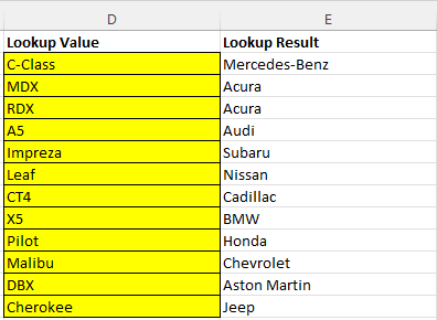
The lookup values are correct but if they get re-sorted, they’re now referencing the wrong values and the lookup results are incorrect:

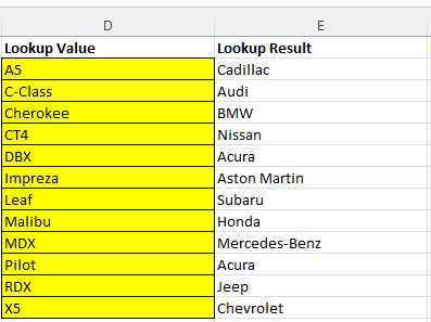
After sorting column D in ascending order, the formula is incorrectly saying that Acura makes the Pilot and that there’s a BMW Cherokee. Here’s what the formula looks like in cell E2 before sorting:

=VLOOKUP(Sheet1!D2,A:B,2,FALSE)

The error is in the sheet reference. Since it’s including Sheet1!D2 instead of just D2, the value isn’t automatically updating when resorting. Excel automatically inserts the sheet referencing if you’re editing a formula and jumping from one sheet to another. The formula is locking that value in place, even when you sort. Getting rid of the sheet references fixes the error.

If you liked this post on 7 Reasons Why VLOOKUP Cannot Find the Right Value, please give this site a like on Facebook and also be sure to check out some of the many templates that we have available for download. You can also follow us on Twitter and YouTube.