How to Use Checkboxes in Google Sheets

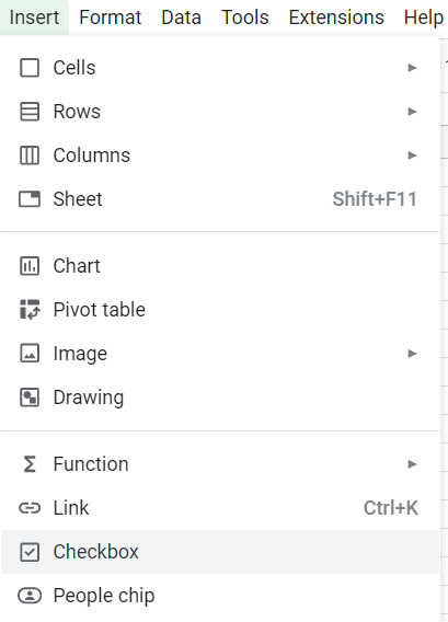
Did you know that you can easily add checkboxes to Google Sheets? In this post, I’ll show you how you can do that. Plus, I’ll share a google sheets script that can automatically update other cells when you tick and untick checkboxes in Google Sheets.

Adding checkboxes to Google Sheets

In Google Sheets, all you need to to do add a checkbox to your sheet is to go to the Insert tab and click on the Checkbox button:

Clicking the button will add a checkbox to the active cell. By default it is unchecked, and selecting the cell will show a value of FALSE in the formula bar. When the checkbox is ticked, then the value changes to TRUE.

Using checkboxes to trigger other calculations

Ticking a checkbox or unticking it doesn’t on its own accomplish anything. However, it could trigger another calculation, with the value being used in a formula. For example, suppose you have a checkbox in cell A1. You could create another formula that looks at if the value is TRUE or FALSE (checked vs unchecked):

=if(A1=TRUE,1,0)

In the above formula, if the checkbox is selected, the formula will return a value of 1. Otherwise, it will be 0. This formula could be modified to do a summation or other something more complex.

Using Google Scripts with checkboxes

Another way you can use checkboxes is with a script that runs when they are checked. Suppose for example you had an inventory sheet and wanted to check off when an item was shipped or received. Clicking the checkbox could populate the date when you checked off the box. With a formula, you wouldn’t have that capability since it would always recalculate. But with a script, it could lock in that value every time the checkbox is ticked or unticked.

To create a script in Google Sheets, you need to go to the Extensions menu and select App Script. The following script will look for changes in the 2nd column (Column B) and if a value is set to TRUE, it will populate the date in the 1st column (Column A). If it’s set to FALSE, then it will clear the value in column A:

function onEdit(e) {
  let range=e.range;
  let activeRow = range.getRow();
  let activeColumn = range.getColumn();
  let cellValue = range.getValue();
  let sheet = SpreadsheetApp.getActiveSheet();


    if (activeColumn == 2) {
      if (cellValue == false) {
          sheet.getRange(activeRow,1).clearContent();
      } else {
          sheet.getRange(activeRow,1).setValue(new Date());
      }
    }
}

Copy that code in its entirety as a new function in the app script. Then, click on the Save button. Now you can go into the spreadsheet and try it out. If you want to change any of the columns, you can change either the active column from B (replace the number 2 in the code above) or where the date value gets populated (see the lines of code that reference activeRow,1, which corresponds to the first column, column A).

If you liked this post on How to Use Checkboxes in Google Sheets, please give this site a like on Facebook and also be sure to check out some of the many templates that we have available for download. You can also follow us on Twitter and YouTube.