LoopStocksGoogleSheets

Loop Through Stocks in Google Sheets With a Macro

Google Sheets provides investors with a great way to pull in stock prices, ratios, and all sorts of information related to stocks. Pulling in a stock’s history, for example, can make it easy for you to calculate a stock’s relative strength index, or create a MACD chart. But doing any sort of analysis for multiple stocks at a time isn’t easy. One way around this is to create a macro using Google App script that can automate the process for you and cycle through multiple stocks. Don’t know how to do it? No problem, because below I’ll provide you with a setup and a code that you can use.

First, I’ll go through creating the file from scratch and how it works.

Setting up the template

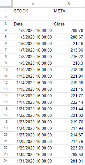
In this example, I’m going to find the stock’s largest value for a specific period. To start, I’m going to use the GOOGLEFINANCE function to get the stock history going back to Jan. 1, 2020. In the below example, I’ve got the price history for Meta Platforms, aka Facebook:

Stock history in Google Sheets for Meta Platforms.

In cell B1 I’ve put a variable for the ticker symbol. This is to avoid hardcoding anything in the formula. This is important to make the process easy to update. In the macro, I’m going to cycle through ticker symbols. In Cell E2, I also have a formula that grabs the largest value in column B (the closing price):

=MAX(B:B)

However, this is where you can put your own formula or the results of your own calculation. Whether it’s a minimum, a maximum, or some other computation you want to do, you can put the results of that calculation here. This is the cell that will get copied during the macro.

Then, in column G, I have a list of the stocks that I want the macro to cycle through:

A list of stocks on Google Sheets.

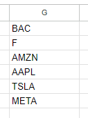
As long as it’s a valid ticker symbol that the GOOGLEFINANCE function recognizes, you can enter it in this column. You can expand it as far as you like. However, if the macro goes on for too long then it will eventually time out and stop. If you want to cycle through every stock in the S&P 500, it is possible, but just be aware that you’ll likely have to do it in chunks. When testing it myself, I estimated I could do somewhere in the neighborhood of 200+ stocks in a single run. Once done, I copied the values onto another place on the spreadsheet with the values, and then replaced the stocks in column G with the next batch.

In Cell J1, I also have a variable called tickercount. This is a helper calculation to make the macro efficient. Instead of it having to count the number of stocks in my list, I provide it for the macro — anything to make it run quicker.

The Apps Script Code

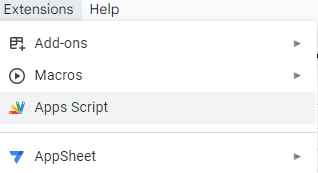
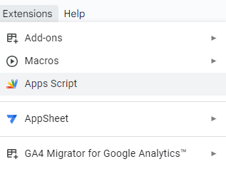
Now it’s time for the code to make this all work. To add code to your Google Sheet, select the Extensions menu and select Apps Script

Selecting Apps Script from Google Sheets.

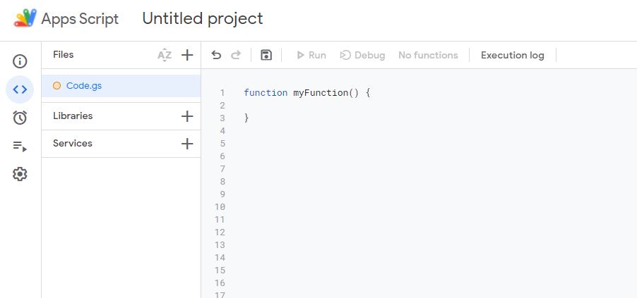
Once in Apps Script, you can setup a new function. You should see the following:

United project in Google Sheets Apps Script.

Here’s the entire code that you can use based on my setup:

function myFunction() {
  
var sht = SpreadsheetApp.getActiveSheet();
var lastrow = sht.getRange("tickercount").getValue();

for (i=1; i<=lastrow;i++) {

  //change ticker
  sht.getRange('B1').setValue(sht.getRange('G' + i).getValue());

  //copy maximum value
  var result = sht.getRange('result').getValue();

  sht.getRange('H' + i).setValue(result);
  

}
}

Here’s a brief explanation of how the code works:

  • It begins by selecting the active sheet.
  • It determines the last value based on the ‘tickercount’ named range.
  • It loops through the values in column G.
  • It takes the value in column G and pastes it into cell B1 (the ticker variable).
  • The macro then gets the value from cell E1 (it has a named range called ‘result’)
  • It pastes the value of the result into column H, to the same row that the stock ticker was on.

If you leave my setup the way it is, what you can do is do any of your desired calculations on another part of the worksheet. As long as it doesn’t interfere with the ticker list or any of the ranges used in the macro, then you’re fine. You can also adjust where the cells are if that makes it easier. For example, you could move the ‘result’ named range from E1 to somewhere else in the spreadsheet. With a named range, you don’t need to worry about updating the cell reference.

Running the macro

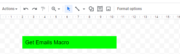
A final part of this macro is actually running it. You need a way to trigger it. In my example, I’m using a button. This makes it easy to see what you need to click on for the macro to run. Here’s how you can create a button in Google Sheets and assign a macro to it:

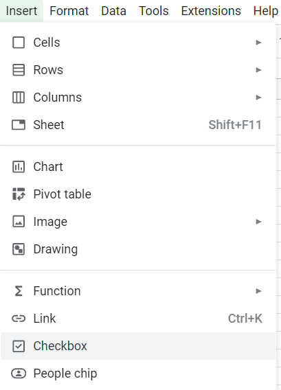
1. Go to Insert and select Drawing

2. Create a shape, add text to it, and whatever colors/formatting you want. Then click Save and Close.

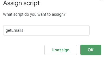
3. Select the button and click on the three dots on the right-hand side, where you will see an option to Assign Script.

4. In the following dialog box, enter the name of your function (don’t include the parentheses). The default function in Apps Script is called myFunction() and if that’s the macro you want to use, then you would just enter myFunction and click on OK.

If everything works, now when you click on your button, the macro will run. Check for any error messages to see if you run into any issues. If you need to edit the button afterwards, right-click on it first so that you don’t accidentally trigger the macro.

One thing to note is that when you run a macro on a Google Sheets file for the first time, you’ll be given a warning about doing so:

Google Sheets warning message.

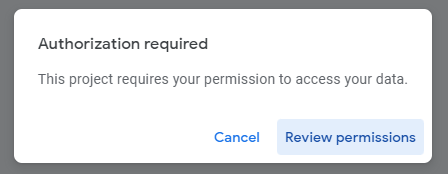
Click on Review permissions and select your Google account. You’ll get the next warning, saying that Google hasn’t verified this app and you’ll need to click on Advanced to continue despite the warnings. This is similar to the warnings you encounter in Microsoft Excel when enabling macros. Once you proceed and click on Allow, the macro will proceed to run.

Here’s how it looks in action:

Download my loop macro template

If you’ve gone through this post and run into issues or it is too complicated for you, feel free to download my loop macro template. Since it’ll create a copy for your use, you can modify it however you like to suit your needs.


If you like this post on Loop Through Stocks in Google Sheets With a Macro, please give this site a like on Facebook and also be sure to check out some of the many templates that we have available for download. You can also follow me on Twitter and YouTube. Also, please consider buying me a coffee if you find my website helpful and would like to support it.

GmailtoSheets

How to Get Emails Into Google Sheets

Did you know that you can pull in emails from your Gmail account into Google Sheets? This can be useful if you don’t want to open up Gmail and do a search; you can do it right within Google Sheets. You can extract the body, subject, and other attributes. This can make it easy to scan through your messages and potentially parse out data from the body. Below, I’ll share with you the code to do this and how it works. You can also download the template if you don’t want to create it yourself.

Creating the sheet and setting up the variables

You probably don’t want to pull every email into your Google Sheets file. For that reason, it’s important to set up variables that will allow you to do a search. In my template, I’ve got an area to search by the subject and by label, with the named ranges being keysubject, and keylabel, respectively. This is where the search terms go. And this is similar to how you would search within Gmail, searching by both the subject and the label.

The Google Apps Script code

To attach the code to your Google Sheets file, you’ll need to go the Extension tab and select the option for Apps Script

Selecting the Apps Script option in Google Sheets.

From there, you should see a new tab open that gives you an untitled project where you can enter in code:

Apps Script code in Google Sheets.

The function name can remain as default, the key is to copy the code within the curly brackets, { and }. The code that I use for the function to pull in emails is as follows:

var ss = SpreadsheetApp;

var sht = ss.getActiveSheet();

var lastrow = sht.getLastRow();

var k = 6;

var rng = sht.getRange(k,1,lastrow,4);

rng.clearContent();

var emailstring = 'https://mail.google.com/mail/u/0/#inbox/';

var emaillink;

var keysubject = "subject:(" + sht.getRange("keysubject").getValue().toString()+")";

var keylabel = sht.getRange("keylabel").getValue().toString();

var searchquery = GmailApp.search(keylabel + " " + keysubject);

var allthreads = GmailApp.getMessagesForThreads(searchquery);

var emaildate;

var emailsubject;

for (var i=0; i<allthreads.length; i++) {

  var activethread = allthreads[i];

  for (var j=0; j<activethread.length; j++) {

            emaildate = activethread[j].getDate();

            emailsubject = activethread[j].getSubject();

            emailbody = activethread[j].getPlainBody().substring(0,300);

            emailID = activethread[j].getId();

            sht.getRange(k,1).setValue(emaildate);

            sht.getRange(k,2).setValue(emailsubject);

            emaillink = emailstring + emailID

            sht.getRange(k,3).setValue(emaillink);

            sht.getRange(k,4).setValue(emailbody);

          k +=1

  }

}

There are a couple things to note in the code, should you want to change the layout of your file and where you want the data to go.

At the beginning of the code, there is a variable, k. It determines the starting row for the data. In my code, the value is set to 6 because my headers are in row 5. That means row 6 is the starting point for the data. If you want your headers to be in row 10, for example, you’ll want to set the k value to 11, so that it starts on the following row.

Towards the end of the code, you’ll see where the values are being populated. For example, the date of the email is being populated with the following line:

            sht.getRange(k,1).setValue(emaildate);

The k variable is specified at the beginning of the code. However, you can change the the column number (1) at this line. Do not change the k value here. If you do, then your data will be overwritten in the same row over and over. This is because in this part of the code the function is doing a loop and it will increment the k value. And so if you want to change it, you need to do it when the k variable is first set up — before the loop.

If, however, you want to change the column that the value is going to, this is the correct place to do so. For example, suppose you don’t want the date going into column A, then you can change the column number. For example, if you want to change it to column B, then you would change (k,1) to (k,2).

If there are certain fields that you don’t want to be populating, then you can also just remove those lines entirely.

For the body of the email, you may want to adjust how much of it gets pulled into the file. Too much text can force your column to get spread out. And if there are line breaks, the row can also get expanded. In my code, I’ve set the limit to the first 300 characters. However, you can change that by adjusting the following line of code:

emailbody = activethread[j].getPlainBody().substring(0,300);

One last note before moving on from this section — remember to save any changes before trying to run the macro again. If you don’t save, then the changes won’t be applied when you run the macro.

Adding a button to trigger the macro

The one thing that you may want to do after adding the code is to create a button on your spreadsheet to trigger it. Otherwise, you’ll need to go to the Apps Script tab and click the run button each time, which isn’t practical.

Instead of doing that, select the Insert button on the Google Sheets file and select Drawing. You’ll have a blank canvas where you can create a button. Here, you can select an option to create a shape and enter text within it. You can apply different colors to also make it stand out. One you’re done designing it, click on Save and close and the button will be on your spreadsheet.

Creating a button in Google Sheets.

Once it’s within your spreadsheet, you’ll see that there will be three dots off to the right of the button. This is where you can assign your button to the macro that you’ve created. In my example, my function is called getEmails and that’s what I’ll enter when I’m assigning the button to a script;

Assigning a script to a button.

If you’ve used a different function name, you will need to enter it above, and then click OK. Don’t enter the parentheses, (), which come after the function in Apps Script. Once you’ve assigned the script to the button, you can now click on the button and run the function.

This will only run on the email account you’re logged in on

If you’re like me and you have multiple Gmail accounts, the one thing you need to know is that this will macro will run on the account you’re logged in on; it won’t be able to toggle between different accounts for you.

Download the file

You can set up this file yourself but if you prefer to just use the version I’ve created, you can download a copy of my template here.


If you liked this post on How to Get Emails Into Google Sheets, please give this site a like on Facebook and also be sure to check out some of the many templates that we have available for download. You can also follow me on Twitter and YouTube. Also, please consider buying me a coffee if you find my website helpful and would like to support it.

H2Echeckboxes

How to Use Checkboxes in Google Sheets

Did you know that you can easily add checkboxes to Google Sheets? In this post, I’ll show you how you can do that. Plus, I’ll share a google sheets script that can automatically update other cells when you tick and untick checkboxes in Google Sheets.

Adding checkboxes to Google Sheets

In Google Sheets, all you need to to do add a checkbox to your sheet is to go to the Insert tab and click on the Checkbox button:

Adding a checkbox in Google Sheets.

Clicking the button will add a checkbox to the active cell. By default it is unchecked, and selecting the cell will show a value of FALSE in the formula bar. When the checkbox is ticked, then the value changes to TRUE.

Using checkboxes to trigger other calculations

Ticking a checkbox or unticking it doesn’t on its own accomplish anything. However, it could trigger another calculation, with the value being used in a formula. For example, suppose you have a checkbox in cell A1. You could create another formula that looks at if the value is TRUE or FALSE (checked vs unchecked):

=if(A1=TRUE,1,0)

In the above formula, if the checkbox is selected, the formula will return a value of 1. Otherwise, it will be 0. This formula could be modified to do a summation or other something more complex.

Using Google Scripts with checkboxes

Another way you can use checkboxes is with a script that runs when they are checked. Suppose for example you had an inventory sheet and wanted to check off when an item was shipped or received. Clicking the checkbox could populate the date when you checked off the box. With a formula, you wouldn’t have that capability since it would always recalculate. But with a script, it could lock in that value every time the checkbox is ticked or unticked.

To create a script in Google Sheets, you need to go to the Extensions menu and select App Script. The following script will look for changes in the 2nd column (Column B) and if a value is set to TRUE, it will populate the date in the 1st column (Column A). If it’s set to FALSE, then it will clear the value in column A:

function onEdit(e) {
  let range=e.range;
  let activeRow = range.getRow();
  let activeColumn = range.getColumn();
  let cellValue = range.getValue();
  let sheet = SpreadsheetApp.getActiveSheet();


    if (activeColumn == 2) {
      if (cellValue == false) {
          sheet.getRange(activeRow,1).clearContent();
      } else {
          sheet.getRange(activeRow,1).setValue(new Date());
      }
    }
}

Copy that code in its entirety as a new function in the app script. Then, click on the Save button. Now you can go into the spreadsheet and try it out. If you want to change any of the columns, you can change either the active column from B (replace the number 2 in the code above) or where the date value gets populated (see the lines of code that reference activeRow,1, which corresponds to the first column, column A).


If you liked this post on How to Use Checkboxes in Google Sheets, please give this site a like on Facebook and also be sure to check out some of the many templates that we have available for download. You can also follow us on Twitter and YouTube.