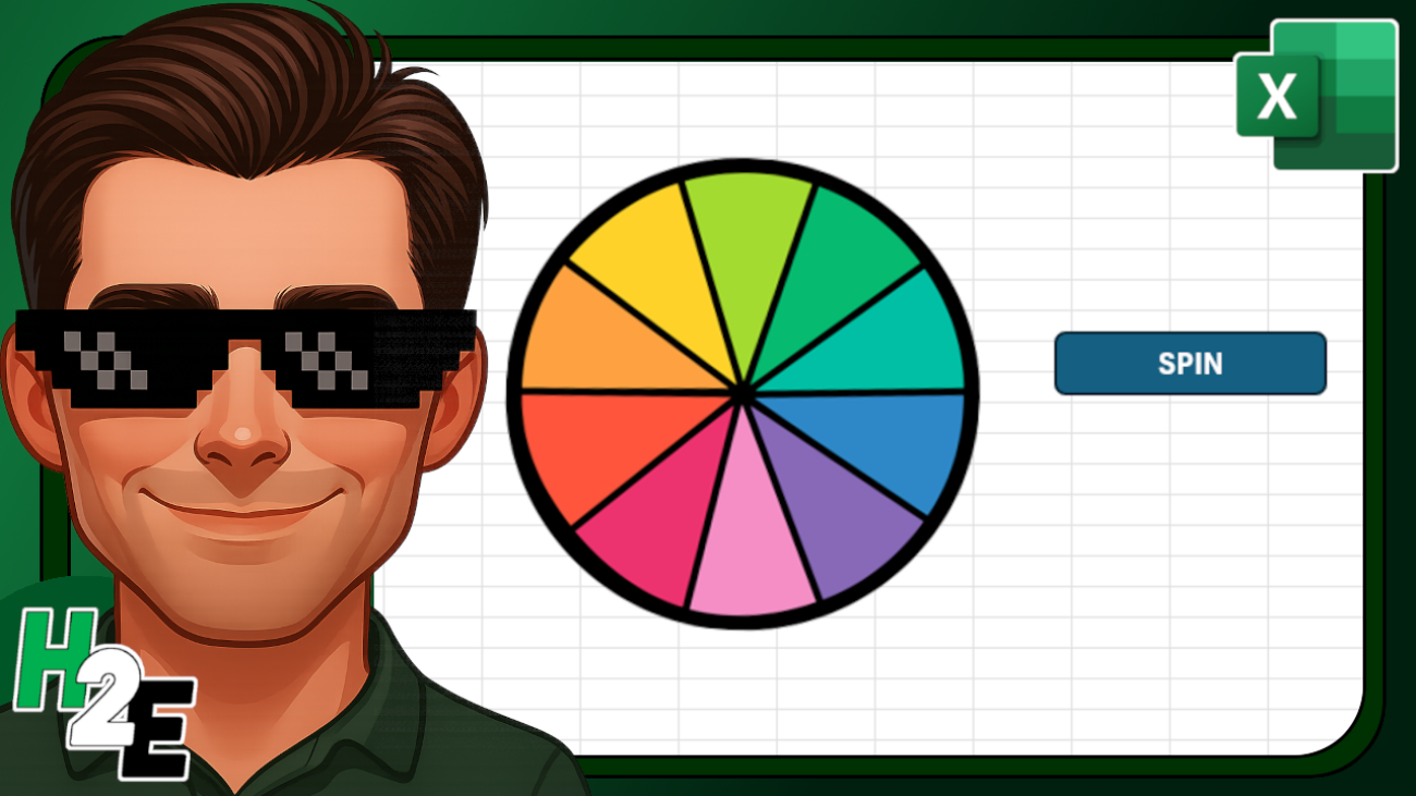
Do you want to create a spinning wheel like in the video below?
In this post, I’ll show you how you can do this, with the help of visual basic. There are a couple of ways you can create a spinning wheel effect. I’ll go over both approaches, and share the code with you so that you can set it up in your own spreadsheet.
Create a spinning wheel effect by rotating an object
The easiest way to spin a wheel, or any object for that matter, is to rotate it. This can be done in visual basic. Before you get started, however, you need to know the name of the shape that you want to spin.
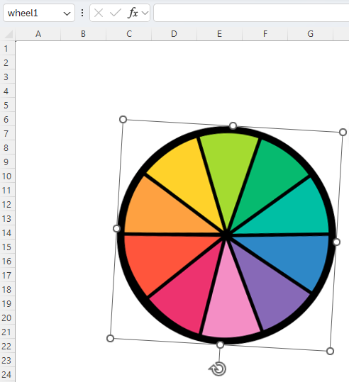
In the above screenshot, I have inserted a wheel into my spreadsheet, but you can use any image. In the top-left-hand corner, you’ll notice it says wheel1 — this is the name of the object. You change this to whatever you want. However, this is what you’ll need to reference in the macro when applying the spin effect.
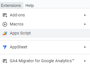
Now, go into visual basic. This can be done using ALT+F11 shortcut. Then, you’ll need to go to the Insert option from the menu and click on Module.
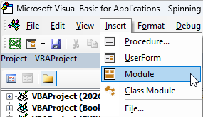
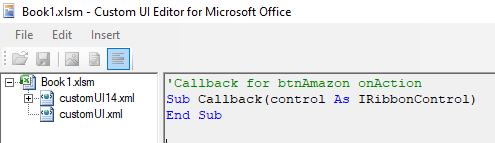
Then in Module 1, copy the following code in:
Sub SpinEffect()
    Dim i As Long
    Dim wheel As Shape
    Set wheel = ActiveSheet.Shapes("wheel1")

     For i = 1 To 100 Step 1
        wheel.IncrementRotation 5
        DoEvents
    Next i


     For i = 1 To 100 Step 1
        wheel.IncrementRotation 3
        DoEvents
    Next i


     For i = 1 To 100 Step 1
        wheel.IncrementRotation 2
        DoEvents
    Next i


     For i = 1 To 500 Step 1
        wheel.IncrementRotation 1
        DoEvents
    Next i
End Sub
At the beginning of the code, I specify the name of my object — wheel1. This is where you need to update the code to reflect the name of your object.
The rest of the code is going through a series of loops. The first one is rotating the image by 5 degrees, then 3 degrees, then 2, and finally 1. The last loop goes through 500 steps and is the longest. You can adjust these to change the speed of the wheel’s rotation.
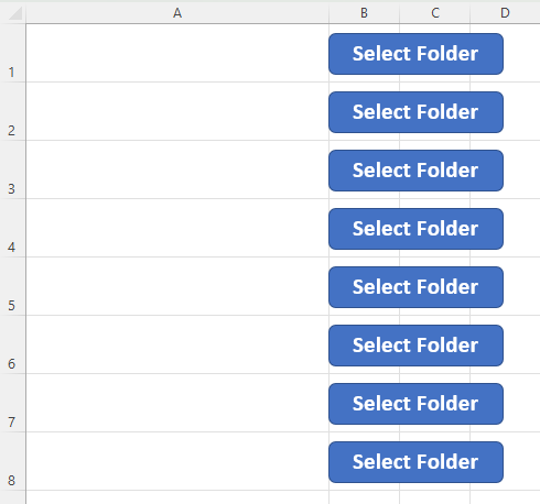
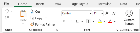
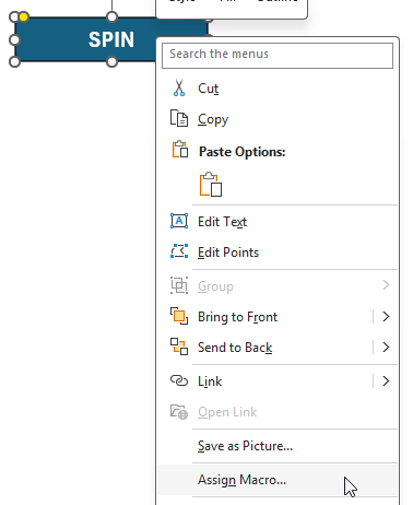
You can also insert a shape that links to this macro, so that it effectively becomes a button. In my example, I created a rectangle and added the text ‘SPIN’ onto it. If you go to the Insert menu on the Excel ribbon and select Shapes, you can create your own.
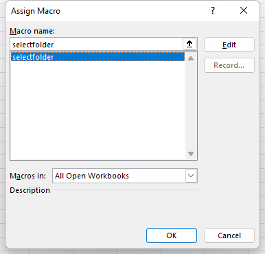
Once you’ve created a shape, you can assign a macro to it by right-clicking on the shape and selecting Assign Macro.
Then, select your macro and click on OK.
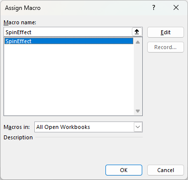
Now, anytime you click on the button, the macro will run, and your object will spin.
The one limitation about this method is that there is no way to know which value your wheel landed on. It spins, but there is no easy way to determine what it landed on. This is where the second method comes into play.
Creating a spin effect by changing visibility
This method is a bit more complex, but it addresses the main issues from the first approach, which is that you’ll known which value was selected.
I’m going to use the same wheel, but this time I’m going to make nine copies of it — one for each possible outcome. I will do the rotations myself and then just toggle the visibility using code. The setup can be a bit more tedious here because you’ll need to make sure the objects are on top of one another and that the rotations are precisely in the right position.
You’ll have to do this for each rotation and each object. You’ll also want to name each individual object so that you know which value it corresponds to.
Once the objects are all aligned, then you can insert the following code:
#If VBA7 Then
    Public Declare PtrSafe Sub Sleep Lib "kernel32" (ByVal dwMilliseconds As LongPtr)
#Else
    Public Declare Sub Sleep Lib "kernel32" (ByVal dwMilliseconds As Long)
#End If

Sub spin()

Dim wheel1 As Shape
Dim wheel2 As Shape
Dim wheel3 As Shape
Dim wheel4 As Shape
Dim wheel5 As Shape
Dim wheel6 As Shape
Dim wheel7 As Shape
Dim wheel8 As Shape
Dim wheel9 As Shape
Dim wheel10 As Shape

Set wheel1 = ActiveSheet.Shapes("wheel1")
Set wheel2 = ActiveSheet.Shapes("wheel2")
Set wheel3 = ActiveSheet.Shapes("wheel3")
Set wheel4 = ActiveSheet.Shapes("wheel4")
Set wheel5 = ActiveSheet.Shapes("wheel5")
Set wheel6 = ActiveSheet.Shapes("wheel6")
Set wheel7 = ActiveSheet.Shapes("wheel7")
Set wheel8 = ActiveSheet.Shapes("wheel8")
Set wheel9 = ActiveSheet.Shapes("wheel9")
Set wheel10 = ActiveSheet.Shapes("wheel10")

Dim i As Integer, j As Integer, cycle As Integer
    Dim winningNumber As Integer
    Dim delay As Long

    winningNumber = Int((9 * Rnd) + 1)

    ' 1. Initial Reset
    For i = 1 To 10
        ActiveSheet.Shapes("wheel" & i).Visible = msoFalse
    Next i

    ' --- STAGE 1: FAST (10 Cycles) ---
    delay = 10
    For cycle = 1 To 10
        For j = 1 To 10
            ActiveSheet.Shapes("wheel" & j).Visible = msoTrue
            DoEvents
            Sleep delay
            ActiveSheet.Shapes("wheel" & j).Visible = msoFalse
        Next j
    Next cycle

    ' --- STAGE 2: MEDIUM (10 Cycles) ---
    delay = 30
    For cycle = 1 To 10
        For j = 1 To 10
            ActiveSheet.Shapes("wheel" & j).Visible = msoTrue
            DoEvents
            Sleep delay
            ActiveSheet.Shapes("wheel" & j).Visible = msoFalse
        Next j
    Next cycle

    ' --- STAGE 3: SLOW (10 Cycles) ---
    delay = 40
    For cycle = 1 To 10
        For j = 1 To 10
            ActiveSheet.Shapes("wheel" & j).Visible = msoTrue
            DoEvents
            Sleep delay
            ActiveSheet.Shapes("wheel" & j).Visible = msoFalse
        Next j
    Next cycle


    ' --- STAGE 4: SLOW (10 Cycles) ---
    delay = 50
    For cycle = 1 To 10
        For j = 1 To 10
            ActiveSheet.Shapes("wheel" & j).Visible = msoTrue
            DoEvents
            Sleep delay
            ActiveSheet.Shapes("wheel" & j).Visible = msoFalse
        Next j
    Next cycle


    ' --- STAGE 5: SLOW (10 Cycles) ---
    delay = 60
    For cycle = 1 To 10
        For j = 1 To 10
            ActiveSheet.Shapes("wheel" & j).Visible = msoTrue
            DoEvents
            Sleep delay
            ActiveSheet.Shapes("wheel" & j).Visible = msoFalse
        Next j
    Next cycle


    ' --- FINAL LAP: STOP ON WINNER ---
    ' Even slower for the "crawl" to the finish line
    delay = 70
    For j = 1 To winningNumber
        ActiveSheet.Shapes("wheel" & j).Visible = msoTrue
        DoEvents
        Sleep delay

        ' Only hide if it's not the final winning shape
        If j < winningNumber Then
            ActiveSheet.Shapes("wheel" & j).Visible = msoFalse
        End If
    Next j

    MsgBox "The wheel stopped on Wheel " & winningNumber & "!"

End Sub
This code is longer and how it works is it determines the winning value at the beginning, based on a random number generator. Then the macro goes through loops to change the visibility of all the wheels, eventually revealing the winning one at the end.
If you liked this post on How to Create a Spinning Wheel in Excel, please give this site a like on Facebook and also be sure to check out some of the many templates that we have available for download. You can also follow me on X and YouTube. Also, please consider buying me a coffee if you find my website helpful and would like to support it.