GetFinancials2

How to Download Financial Statements Into Excel and Google Sheets

In a previous post, I went over how to download a company’s financial statements from the Wall Street Journal’s website. However, that connection appears to now be closed. One of the risks when using Power Query to download data from a website that the connection will always be there. But there is another way to get financial statement data, and it can allow you to download much more than what was available through the Wall Street Journal.

You’ll need to setup an account with Alpha Vantage

The website that you can use is Alpha Vantage. It provides API access which you can use to download financial data. There is a free account but there is a limit to the number of requests you can make every day — up to 25. But with the wealth of information you can get with just a single query, there’s a lot of data you can accumulate.

Once you sign up for an account with Alpha Vantage, you’ll have an API key that you can use to connect to its database. You’ll need to save that key to download the data.

Use the site’s custom Excel add-in

Once you have the API key, you can start downloading data. But rather than creating your own template or even using Power Query, what you can do is download the sample Excel files that are available on the site on the spreadsheets page. Here you can select to download the Office 365 add-on, which also includes sample Excel files that can get you started in seconds.

There is a template called FundamentalData.xlsx which contains a file that’s ready to go to import the financials. When you first open it, you’ll need to select the AlphaVantage(Web) tab and click on the Open Taskpane command.

The alphavantage tab in Excel.

From there, you’ll see an option to input your API Key.
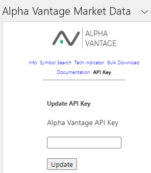
The alphavantage API key section.

Then, on the filings tab, you’ll see an area where you can specify the ticker symbol you want, the type of filing (cash flow, income statement, or balance sheet) and the reporting frequency (quarterly versus annual). Then, as you make your selections, the data on your spreadsheet will update with various financial metrics.
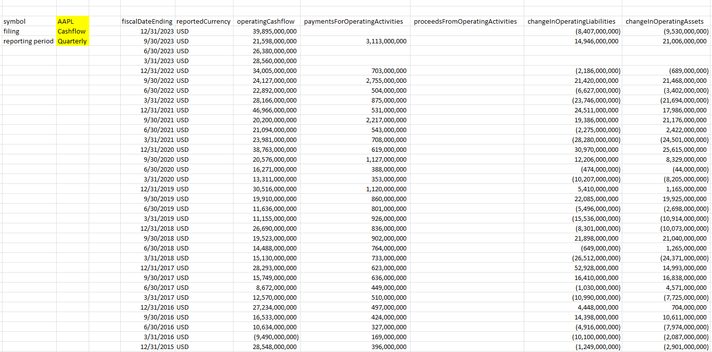
Downloading financial statement data in Excel.

Using Alpha Vantage is one of the better options for investors today who want to download financial data into Excel.

Importing financial statement data in Google Sheets

The company also has a Google Sheets add-on available from the Google Workspace Marketplace, just go to Extensions ->Add-ons -> Get add-ons. Then search for ‘Alpha Vantage’ and download the add-on:

The Alpha Vantage add-on in Google Sheets.

Once installed, go back to the Extensions menu, select Alpha Vantage Market Data and select Enter API Key, where you can paste your API key into. Once that’s done, you can use formulas to pull in financials. The following pulls in the quarterly income statement data for MSFT stock:

=AVGetCompanyFilings(“MSFT”,”IncomeStatement”,”Quarterly”)

For a full breakdown of what you can download on Google Sheets, refer to the documentation on the Alpha Vantage website.

Download the data using Power Query

If you prefer not to install an add-in, then you can still download the data from Alpha Vantage using Power Query. You can refer to the documentation for the various links to pull financial data. For the income statement, for example, this is the following url:

https://www.alphavantage.co/query?function=INCOME_STATEMENT&symbol=TICKER&apikey=DEMO

Where Ticker is the stock symbol and Demo is your API Key. To generate the data in Power Query, use the Get Data option and select From Web and paste the URL into there:

Using Power Query to download financial statement data.

Then, once Power Query is loaded up you have the option to specify whether you want the list for the annual reports or the quarterly reports.
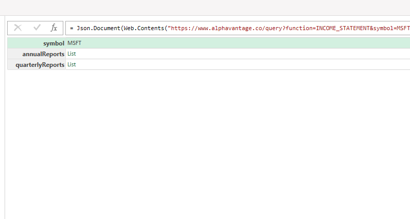
Selecting the type of financial report to download from Power Query.

If I select the quarterlyReports list, I’ll have another list of records. I can expand this by clicking on the Convert To Table button in Power Query:
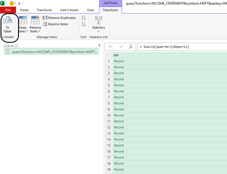
Converting a list of records in Power Query into table.

This will put everything back into a single column. This time, however, I can expand all the fields out by clicking the two arrows going in opposing directions.
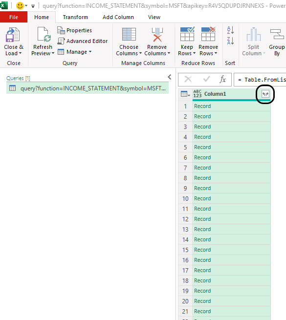
Expanding a column in Power Query to list all the fields.

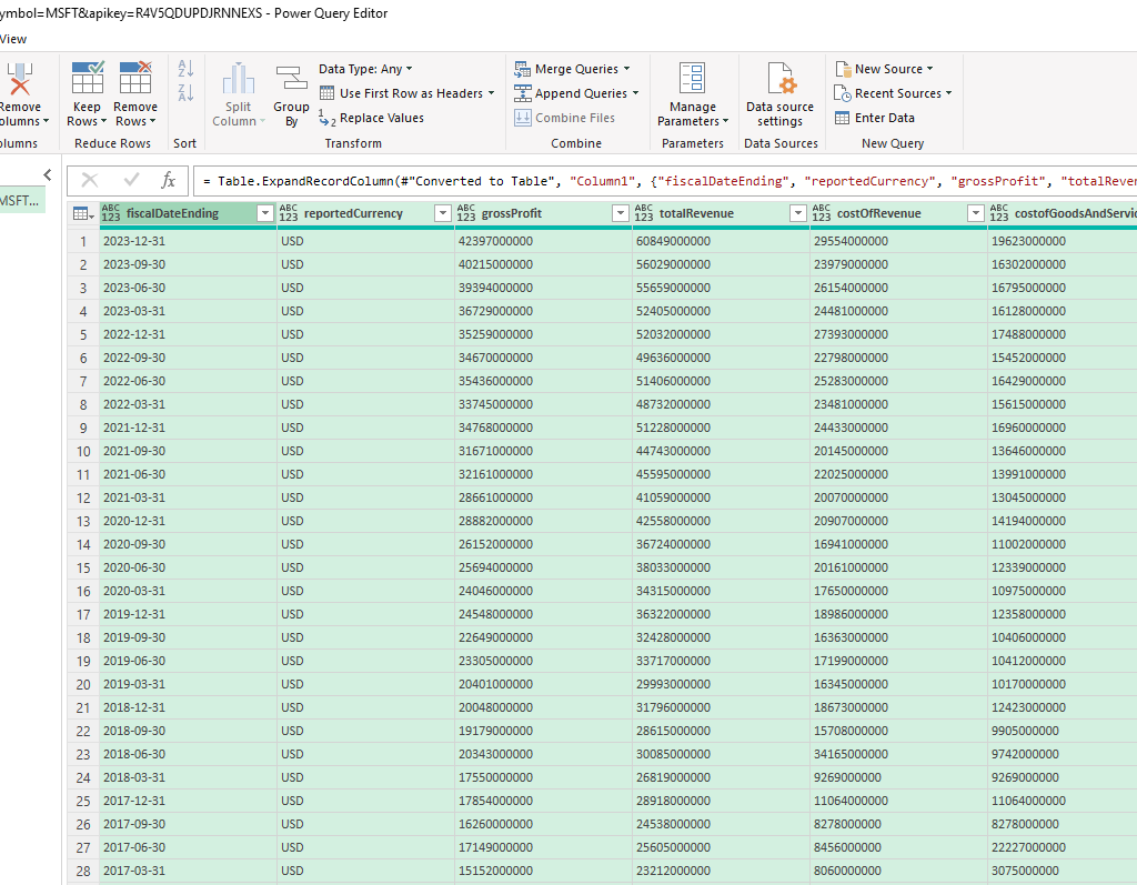
Now my data looks complete:

Income statement data loaded in Power Query.

And this is what it looks like once it’s loaded back into Excel:
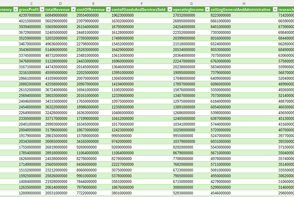
Income statement data loaded into Excel.

If you like this post on How to Import Financial Statements Into Excel and Google Sheets please give this site a like on Facebook and also be sure to check out some of the many templates that we have available for download. You can also follow me on Twitter and YouTube. Also, please consider buying me a coffee if you find my website helpful and would like to support it.

H2EOrganizeTabs

Free Add-In to Organize Your Tabs

Do you have a spreadsheet that has more than 10 tabs? If so, you probably know it can be challenging and time-consuming to organize and move all those sheets around if you want to re-arrange them. Oftentimes it’s just easier to leave them as they are. In this post, I’ll share with you a free Excel add-in I’ve been working on that will make it easy to move tabs around and alphabetize them.

Download and install the add-in

You can download the add-in from this link. Once you’ve downloaded it, go into Excel and select File and then Excel Options. There, you’ll see a section for Add-ins. Click on that and click on the Go button next to Manage Excel Add-ins near the bottom:

Manage excel add-ins button.

You should see a list of available add-ins. To add the one you just downloaded, click on the Browse button on the right-hand side and then select the add-in that you just downloaded. Then you should see it added to your list and the box should be checked off. Once you press OK, you should see the add-in within your Excel spreadsheet, in the middle of your Home tab:

Excel ribbon with the Tab Manager Add-In installed.

The add-in will now be available on all of the Excel files that you open.

Using the add-in

To start using the add-in, click on the Tab Manager button. A form will populate that displays all the tabs in your spreadsheet:

The tab manager launched and ready to use.

To move sheets around, select a sheet and use the arrow keys on the right to move them either up or down. Once you have the order you want, click on the button to Update List and your sheets will be re-arranged.

There’s also an option at the top of the form to Alphabetize the list. Clicking on the button will arrange the sheets in alphabetical order. You can make changes afterward, or you can click on Update List. The point of the add-in is to make it easy to make changes before running the update. If you don’t want to make any changes, simply click on the ‘X’ in the top-right-hand corner.

If you are moving a sheet far enough on the form that you end up moving onto another page/view and notice that the tab names don’t appear to be refreshed, simply click the up and down arrows to refresh the list.

Don’t need the add-in anymore or want to uninstall it?

If you just wanted to try out the add-in or only needed it for one use and want to uninstall it, you can easily do that. Repeat the steps you took to install the add-in, except this time, since it’s already available, simply uncheck the box for the Tabmanager. This will make it unavailable and it will no longer show up on the ribbon.


If you liked this Free Add-In to Organize Your Tabs, please give this site a like on Facebook and also be sure to check out some of the many templates that we have available for download. You can also follow us on Twitter and YouTube.

H2Edatepicker9001

Free Excel Date Picker Add-In

Are you looking for an easy way to add a date to your Excel spreadsheet? You can download my free date picker add-in for Excel. It is useful if you have a form and you want people to select dates or if you just want an easy way to enter a date without worrying about whether it is in the right format.

***Please note on an earlier version of this add-in (and as reflected in the video), the calendar was designed to pop up next to the active cell. However, due to many issues related to scrolling and possible zooming, and multiple screens, it is now set to open at the top (and in the middle) of the screen***

How the date picker add-in works

To launch the add-in, click on CTRL+SHIFT+Z, which will trigger the following calendar to pop up:

Date picker add-in for Excel.

By default, it will jump to the current month. Clicking on any of the dates will enter the date value into the active cell. You can use the arrow keys on the left or right side to change the months. If you want to jump by years, double-click on the year and just enter the desired year. The calendar will automatically adjust, which will be quicker than if you were to just continue pressing the arrow buttons.

Right now the add-in is a stand-alone but look for it to be included as part of a larger add-in package. If you have any suggestions for other features to include in an add-in, feel free to contact us.

How to install an add-in

You can download the date picker add-in here. Once you’ve saved it, go into Excel and select File -> Options -> Add-ins and then depending on your version, you may see an option at the bottom to go to manager Excel Add-ins:

Manage Excel add-ins button.

Click on the Go button and then you will have a list of add-ins you can install. If you didn’t save the add-in into the default folder where the rest of the Excel add-ins are, you just click the Browse button to find where you saved the file. Then, make sure the add-in is checked off and click OK and it will be ready to go.


If you liked the Date Picker Add-in, please give this site a like on Facebook and also be sure to check out some of the many templates that we have available for download. You can also follow us on Twitter and YouTube.

person fixing a computer

This Macro Converts Your QuickBooks Export Into a Table-Friendly Format

QuickBooks does a good job when it comes to recording sales and doing day-to-day accounting tasks. You may be content with the reports that come out of QuickBooks, too. But if you’re looking for some more in-depth analysis to do of your own or to make your own reports, you’re likely going to want to move that data into Excel. And, unfortunately, the QuickBooks export into Excel can be less than optimal.

With many spaces, subtotals, and a non-tabular format, it’s not a very practical output to use in Excel. If you want to run a pivot table and do some serious analysis in Excel, you first have to clean up the data before being able to use it, and that can be a very tedious and tiresome process.

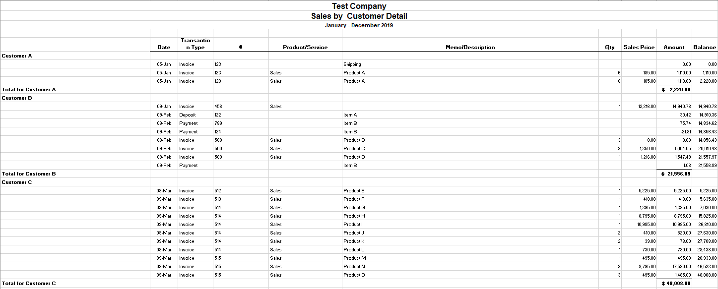
For example, this is what your QuickBooks report might look like when you’re pulling a simple summary of your customer sales:

quickbooks export into excel

There are a lot of things that need to be adjusted for this report to be useable in Excel, including getting rid of the blank spaces and ensuring that the customer information is repeated in the first column, as opposed to just in the first line and in the last line’s total. From afar, it’s a bit of a painful process to have to go in and clean this up. And while it’s not impossible, it’s not going to be quick, either.

That’s where a macro can help you make the task much quicker and it will save you a lot of time if you have to go through these steps often. Click the button on the ribbon and your data will convert into a more table-friendly format! Here’s how it works:

Using the macro to fix the QuickBooks export

Before running the macro, you’ll need to specify the columns where your customer names and dates are:

Then, run the Covert Data button:

Excel button to modify data exported from Quickbooks

Downloading the file

The free version of the QuickBooks macro will allow you to run the conversion if it doesn’t go past 100 rows. However, if you decide to purchase the full version please ensure that the macro and file works as expected. There’s no guarantee the QuickBooks export hasn’t changed or won’t change in the future. If there are changes that need to be made to the macro, please feel free to contact me so that I can make the necessary adjustments. Whether you prefer the add-In or the actual Excel spreadsheet itself, both versions are available both here and in the paid version as well.

Here is the download link for the add-in as well as the Excel file. For the paid versions, please visit the product page.

If you have another program or software that you’d like a similar add-in for, I can help with that as well.


If you liked this post, please give this site a like on Facebook and also be sure to check out some of the many templates that we have available for download. You can also follow us on Twitter and YouTube.

addina

Free Excel Add-In: 20+ Macros to Automate Tasks and Make You More Efficient


This add-in is completely free and includes over 20 macros that I have worked on myself and that I hope will help you. Any feedback is welcome, as well as any suggestions for other macros you would like to see added.

Disclaimer
These macros have not been tested exhaustively so I don’t offer any guarantees that they will work under every possible scenario. However, if you run into any issues please let me know and I will work to correct them. When using macros you should always save your work before executing them, as there is no undo button if something doesn’t go as expected.

If you understand and accept these risks, please feel free to download the file here

Below is an overview of all the different macros in the file.

Toggling Workbook and Worksheet Calculations

For those that work on large spreadsheets, this can make it easy for you to not only turn off and on calculations for a workbook, but for individual worksheets. It will also allow you to see whether or not they are set to on or off.

One of the things people sometimes don’t realize is if you turn off calculations in Excel at the workbook level, that disables it for all other workbooks. The danger is if you switch to another file you’re working on you may not realize calculations are still off, by seeing the toggle and whether it is set to on or off can help prevent that.

If you only need an individual worksheet to be off, you can do that as well. However, note that if the workbook calculations are set to off, then all the worksheet calculations will be off as well, regardless of whether or not they say on or off. Workbook settings will supersede any worksheet settings.

Very Hidden Tabs


Hiding tabs in Excel may seem pointless since even an average user would know that you can right-click and select un-hide. However, not many know that you can set them to be ‘very hidden’ and where right-clicking won’t do anything.

I’ve covered this in a post before here, and in this add-in I’ve made it so that you can easily both hide and unhide very hidden tabs.


Removing Excess Spaces


This macro will delete any trailing, leading, or extra spaces in a cell and will help to clean up your data.

Converting Formulas to Values

In some instances you may want to get rid of your formulas and replace them with their results (values), this macro will do that for you. Just select the cells and click the button and the formulas will be gone.

Converting Numbers to/from Text and Changing Signs

These buttons will allow you to choose whether you want to convert numbers that are stored as text into numbers, switch numbers back into text, or just flip the signs from positive to negative or vice versa.

Filtering Out Zero Values From Tables


If you’ve got a table or pivot table that has a lot of zero values in it that you don’t want to see, this will filter them out. This won’t get rid of errors, just zeros, and for it to work in a table, it assumes that the table will start in column A, otherwise it won’t filter the right column for you. The zero values will be removed from the column where your active cell is, so you have to make sure you’ve got the right cell selected before clicking this button.


Multiplying and Dividing by a Factor of 1,000

This is pretty straightforward and is mainly here since dividing can be helpful if you’re dealing with financials and want to cut down the number of placeholders. Multiplying will simply undo those changes.

Combining Columns

If you have data across multiple columns and want to combine it, you can do that with this macro. You don’t have to select entire columns, it can just be a selection. The columns don’t even have to be right next to one another.


Cycling Through Errors


If you want to find all the errors on the worksheet you’re on, this macro will cycle through all of them for you. You can correct an error, and click the Next button to go onto the next error in the sheet.


Removing Merged Cells

When you’re trying to do data analysis, merged cells can be a nightmare, and this will unmerge the cells and put the value into each of the cells as well.


Protecting Your Data


This will help convert your sensitive data into a random number preceded by a series of X’s. There’s a post here detailing how that process works.


Filtering Pivot Tables

If you’ve got a pivot table and want to select multiple items, it can be a tedious process. This macro will allow you to select what selections you want to filter by and apply them for you. But the first cell in the selection needs to match the field name in the pivot table.


Adjusting the Default Pivot Table Format

One of the more annoying things in Excel is that when you create a pivot table, it defaults to a format that isn’t very useful. This is what the macro will help you do:


Quickly Formatting Pivot Table Fields

If you’ve ever needed to change how fields are formatted in a pivot table you know that simply selecting the column and changing the format is a temporary fix. You need to actually go into the field settings. This macro will do that for you, and will set the settings to either comma or accounting format.

Quickly Extracting Unique Values


There are plenty of ways you can get unique values, but I thought an even easier way would be to select the cells and specify where you want those unique values to be output.

Counting Unique Values

If you just want to quickly count how many unique values are in your selection, this macro will do that for you.

Do a Reverse Lookup

Everyone knows how to do a VLOOKUP, but doing the reverse is another story. Take for example a credit card statement. You could have a lot of detail in the string, but only a certain few characters relate to the actual vendor or detail you want:

Using this lookup function the cells you select will be compared against a list you have specified, and if there are any matches, the corresponding field will be returned:


The result:


If you’re doing this with a lot of cells and have a big list, it could be time consuming, and that’s why I added a progress bar to this macro.

Comparing Sheets

This macro essentially looks at two sheets and tells you what is different, and will highlight the differences in them.


Updating Links

If you want to update the link for a cell, it’s not an easy process and involves you right-clicking on the cell and putting the link in there. This macro will do that step, and for the link it will put the cell’s value there, so if you put in the url you want in the cell and then run the macro on those cells, the links will be updated.

Adding the Location to the Footer

Clicking this button will add the path to the workbook you’re working on into the footer so when you
print it out it’s easy to see where the file is saved.

Protect Your Sensitive Excel Data with This Template and Add-in

One of the challenges sometimes with sending your spreadsheet to someone, whether it’s to review or to make changes to it, is that it contains sensitive information.

So I’ve created a template and add-in that will help you accomplish that.

You can download the template here or if you prefer, the add-in is available here.
Disclaimer: I do not offer any guarantees or promises that this will work perfectly and it’s the responsibility of the user to ensure and confirm that all data is adequately protected as the spreadsheet still requires manual steps from the user.

The template will look like a regular spreadsheet, but with one main difference. On the far right end of the Home tab, you’ll see this button:

If you select the data you want to encrypt, whether it’s a few cells or an entire column, then clicking this button will mask your data. Here’s how it works.

In my spreadsheet, in column A, I have a list of customer names that I want to protect.
If I highlight the range and click on the Encrypt Selection button, what will happen is it will mask the data and create a new tab showing me which customer is mapped to which mask:
After all, masking the data is great, but if you don’t know what the data means, it’s not very helpful. The macro creates a tab called “Mapping Hidden Cells” and it’ll give you a popup warning you to delete this tab before you send the data to anyone. The purpose of this tab is to give you the table, and you can either make note of it or save it somewhere. Either way, you’ll want to delete this afterward, otherwise it would make masking the data pointless.
 
If I return to my main tab I notice that the data is now masked:
 
 
The customer names are now nowhere to be found. At this time I’d like to point out that the masking will only happen to the cells that you selected. If for example I had customer data in a different area and didn’t select it, that data would not have been masked.
 
This is why it is crucial for the user to review the data themselves and validate that the sensitive information has in fact been correctly masked, and that the mapping tab has been deleted.