DatabasesinExcel

Create a Database Entry Form in Excel to Populate a Sheet Using VBA Macros

Excel isn’t a database software but as long as you don’t need to manage millions of data points or have complex, interlocking systems, it can potentially do the job for you — and save you plenty of money. You can create forms, that with the use of visual basic, can populate a database which you can track within Excel and then create reports on later.

Designing a user form and database sheet

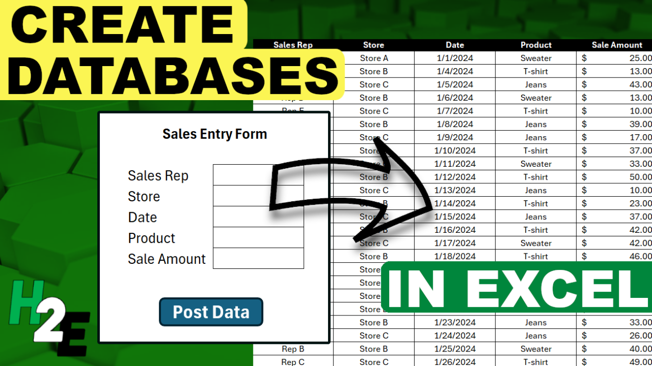
Let’s suppose we want to track sales and commission data. A form that someone may fill out could include the following fields:

  • Sales Rep
  • Store
  • Date
  • Product
  • Sale Amount

Upon entering this data, a user could click on a button to post the data to another sheet within the workbook, thereby adding it to a database. And with more entries, the data can grow over size. We could then use the data to run reports on and to track store sales, calculate commission, and other metrics.

Here’s how I’ve designed this form in Excel:
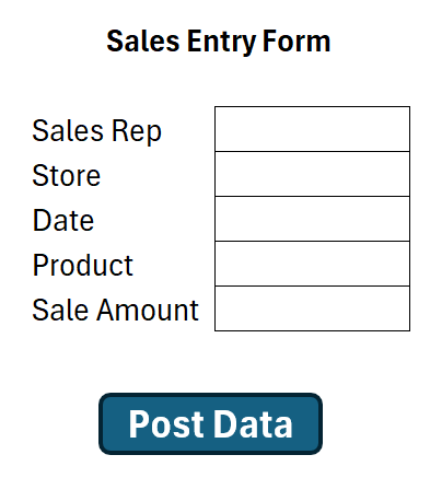
A sales entry form in Excel.

The ‘Post Data’ button was created using a shape. And it will be attached to a macro, which will then post to the database worksheet.

Next, I’ll create the corresponding fields where these values will post to on a separate sheet, which I’ll call the database sheet. The layout is a simple one which just involves the same headers from the sales entry form.

A database sheet contain the fields from the data entry form.

Populating the database sheet using a macro

Next, I’ll create a macro to copy the data from the sales entry form to the next row in the database sheet.

The following macro will find the next row in the database sheet, and then copy the values from the sales entry form into the corresponding field. I’ve also added a message box at the end to let the user know that the data was posted successfully to the database sheet. My inputs in cells C4:C8.

Sub copyinputs()

Dim cl As Range
Dim nextrow As Double
Dim wsinput As Worksheet
Dim wsdatabase As Worksheet

'set the worksheet variables
Set wsinput = Worksheets("Input")
Set wsdatabase = Worksheets("Database")

'detect the next available row based on values in column A
nextrow = WorksheetFunction.CountA(wsdatabase.Range("A:A")) + 1

'copy values over
wsinput.Range("C4").Copy wsdatabase.Range("A" & nextrow) ' copy the sales rep
wsinput.Range("C5").Copy wsdatabase.Range("B" & nextrow) ' copy the store
wsinput.Range("C6").Copy wsdatabase.Range("C" & nextrow) ' copy the date value
wsinput.Range("C7").Copy wsdatabase.Range("D" & nextrow) ' copy the product
wsinput.Range("C8").Copy wsdatabase.Range("E" & nextrow) ' copy the sale amount

MsgBox "Posted!"

End Sub

This macro, called copyinputs still needs to be assigned to the button. To do this, I need to right-click on the button on the sales entry form and select Assign Macro and then select this macro. After doing this, I can start entering data and populating my database. When I finish filling in my data and I click on the Post Data button, I get a message saying it has been posted.
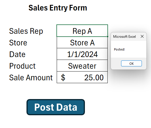
Entering data on the sales entry form in Excel.

And in my database sheet, it has begun populating the data:

Database sheet in Excel containing data from the input page.

As I enter data and click on the Post Data button, it continues adding to my database:

The database sheet growing in size.

Since it is always calculating the next row, it isn’t overwriting the existing information.

Additional macros to setup

This current macro is a simple one which just posts the data. It doesn’t do anything besides that. It doesn’t check for if the fields are entered nor does it clear them after they’ve been entered. You can adjust this, however, to make the macro and form more robust.

Here’s a macro which includes the existing code plus code to clear the values after they’ve been entered, assuming the values are in the range C4:C8.

Sub copyinputs()

Dim cl As Range
Dim nextrow As Double
Dim wsinput As Worksheet
Dim wsdatabase As Worksheet

'set the worksheet variables
Set wsinput = Worksheets("Input")
Set wsdatabase = Worksheets("Database")

'detect the next available row based on values in column A
nextrow = WorksheetFunction.CountA(wsdatabase.Range("A:A")) + 1

'copy values over
wsinput.Range("C4").Copy wsdatabase.Range("A" & nextrow) ' copy the sales rep
wsinput.Range("C5").Copy wsdatabase.Range("B" & nextrow) ' copy the store
wsinput.Range("C6").Copy wsdatabase.Range("C" & nextrow) ' copy the date value
wsinput.Range("C7").Copy wsdatabase.Range("D" & nextrow) ' copy the product
wsinput.Range("C8").Copy wsdatabase.Range("E" & nextrow) ' copy the sale amount

'clear the data
wsinput.Range("C4:C8").ClearContents

MsgBox "Posted!"


End Sub

Additionally, we can setup rules to make sure that the fields have to be entered fully before clicking on the Post Data button. This can prevent incomplete entries from being posted to the database sheet. Here’s how we can add a code to check if the sales rep field contains a value. This can be repeated for all other required fields:

Sub copyinputs()

Dim cl As Range
Dim nextrow As Double
Dim wsinput As Worksheet
Dim wsdatabase As Worksheet

'set the worksheet variables
Set wsinput = Worksheets("Input")
Set wsdatabase = Worksheets("Database")

'detect the next available row based on values in column A
nextrow = WorksheetFunction.CountA(wsdatabase.Range("A:A")) + 1

'check if the sales rep field contains a value
If wsinput.Range("C4") = "" Then
    MsgBox "Please enter a sales rep"
    Exit Sub
End If


'copy values over
wsinput.Range("C4").Copy wsdatabase.Range("A" & nextrow) ' copy the sales rep
wsinput.Range("C5").Copy wsdatabase.Range("B" & nextrow) ' copy the store
wsinput.Range("C6").Copy wsdatabase.Range("C" & nextrow) ' copy the date value
wsinput.Range("C7").Copy wsdatabase.Range("D" & nextrow) ' copy the product
wsinput.Range("C8").Copy wsdatabase.Range("E" & nextrow) ' copy the sale amount

'clear the data
wsinput.Range("C4:C8").ClearContents

MsgBox "Posted!"


End Sub


If you like this post on Create a Database Entry Form in Excel to Populate a Sheet Using VBA Macros please give this site a like on Facebook and also be sure to check out some of the many templates that we have available for download. You can also follow me on Twitter and YouTube. Also, please consider buying me a coffee if you find my website helpful and would like to support it.

StaticDateStamps

Adding Static Timestamps in Excel Using Checkboxes

One way to enhance your spreadsheets is by adding checkboxes. Using checkboxes, you can make data entry easier for your users. And you can create formulas based on whether a checkbox is checked off or not. In the latest version of Excel, using Microsoft 365, it’s easier than ever to create multiple checkboxes in just seconds. And using checkboxes, you can also create timestamps that won’t change.

How to add checkboxes to your Excel spreadsheet in seconds

In Excel’s latest version, a checkbox can be added right from the Insert tab on the ribbon. Simply clicking on the checkbox button will insert a checkbox into your spreadsheet. To insert multiple checkboxes at once, first select all the cells which you want to contain checkboxes. Then, click on the checkbox button. The cells will now be filled with checkboxes.

Using checkbox selections in formulas

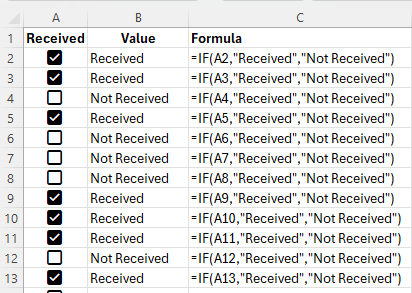
If a checkbox is selected, its value becomes TRUE, and FALSE if it is unchecked. Using an IF function, I can create a formula to check whether the value is TRUE or not, and based on that, determine the output. In the following example, I use checkboxes to determine if something has been received. If it is checked off, then the value is “Received” and if it’s not, then it will say “Not Received”

Excel spreadsheet using checkboxes to determine if something was received or not.

The formula is a straightforward and can be used to track whether something has been processed or not.

Creating a static timestamp in Excel using a checkbox

Let’s use a more complex situation in Excel, such as when we want to lock in the time of when someone received the order, not simply whether or not they received it. This involves a bit more complexity and we’ll need to allow for some circular references in this case, which is usually a no-no in Excel.

Here’s how we can get this scenario to work. Assuming the checkboxes are still in column A, the formula for cell B2 would be as follows:

=IF(A2,IF(B2=””,NOW(),B2),””)

The first argument in the IF statement checks to see if the checkbox is selected. It looks at A2 to see if it returns a value of TRUE or FALSE. Since it is a boolean argument, it is not necessary to state A2=TRUE; that goes without saying in this example.

If that condition is met, we move on to the next IF function. This one checks if B2 (the current cell, and thus, creating a circular reference) is blank. If it is, then the current date and time would be inserted with the NOW function. If it isn’t blank, then the value in B2 would remain as it is. And if the checkbox is A2 isn’t checked off at all, the value in B2 will be blank.

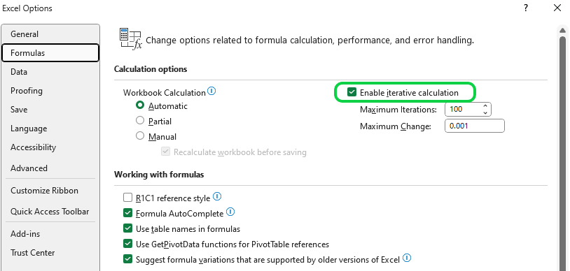
This formula initially won’t work and will give you an error stating that you’ve created a circular reference. To fix this, you need to allow for Iterative Calculations. This will ensure that Excel stops calculating after a certain number of attempts and take the last value. To activate this, go into Excel Options and under Formulas, select to Enable iterative calculation:

Enabling iterative calculations in Excel.

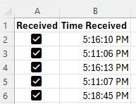
You can leave the default number of iterations. Now, your formula will calculate without the circular reference error. And when you check off boxes, the timestamps will all remain static until the checkboxes become unchecked again.

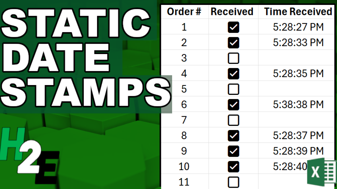
Checkboxes in Excel showing the time received.

In the above screenshot I only show time, but that’s because I have formatted it to only show time. Since the NOW function contains both date and time, you can choose to show both, or just time or date individually.

The drawbacks of iterative calculations

Before you enable iterative calculations, however, you should consider the risks with doing so:

Performance Issues. Iterative calculations can significantly slow down Excel, especially in large and complex worksheets. Excel has to repeatedly recalculate formulas until either the maximum number of iterations is reached or the difference between the results of two calculations is below a certain threshold. This can be particularly noticeable if the workbook contains many formulas or data points.

Accuracy and Precision. The result of an iterative calculation can depend on the maximum number of iterations and the maximum change settings. If these are not appropriately set, the result may be inaccurate or not precise enough for your needs. This is because the calculation stops once the set limits are reached, not necessarily when the correct or most accurate result is found.

Risk of Other Circular Reference Errors. While iterative calculations allow you to use circular references intentionally, they also increase the risk of unintended circular references. Unintended circular references can lead to errors and incorrect data, making it difficult to debug and correct issues within your workbook.

Compatibility Issues. If you share your Excel workbook with users who have iterative calculations disabled, or if the workbook is opened in a different spreadsheet program that doesn’t support iterative calculations, the intended functionality may not work correctly. This can lead to errors or data inconsistency.

Potential for Infinite Loops. Incorrectly configured iterative calculations can lead to infinite loops, where Excel continuously recalculates without reaching a conclusion. This can cause Excel to freeze or crash, potentially leading to data loss if changes haven’t been saved.

As long as you understand the risks of enabling iterative calculations, they can help you in setting static date and time stamps in Excel.


If you like this post on Adding Static Timestamps in Excel Using Checkboxes please give this site a like on Facebook and also be sure to check out some of the many templates that we have available for download. You can also follow me on Twitter and YouTube. Also, please consider buying me a coffee if you find my website helpful and would like to support it.
ExcelDatabase1

Can You Use Excel as a Database?

Microsoft Excel is a powerful spreadsheet software that people use for data analysis, calculations, and reporting. While Excel is primarily designed for managing and manipulating tabular data, many users have explored using it as a database. In this article, I will go over the pros and cons of using Excel as a database, highlighting its limitations and advantages compared to SQL and other alternatives.

Benefits of using Excel as a database

1. Familiarity and Accessibility

Excel enjoys widespread usage, and millions of users are already familiar with its interface and basic functionalities. It is easily accessible and requires no additional software or technical expertise to get started. This means no costly support bills as there are many users all over the world who can provide expertise on spreadsheets. And it’s already included in Microsoft 365, which many businesses already pay for.

2. Quick and Easy Data Entry

Excel provides a user-friendly environment for entering and editing data. Its intuitive grid layout allows for easy data input, and its familiar formula syntax enables simple calculations and data manipulation. You can also create templates for data entry so that it is customized to your company’s needs. Through userforms and visual basic, you can even create wizards that walk users through personalized data entry screens.

3. Simple Sorting and Filtering

Excel offers basic sorting and filtering capabilities that can be helpful for simple data analysis and organization. Users can sort and filter data based on specific criteria to extract relevant information quickly. This can make it easy to review and analyze data on-the-fly. Slicers also add convenience and can make filtering options even easier, giving users the ability to quickly apply filters with just a few clicks of a mouse.

4. Flexible Data Visualization

Excel provides various charting and graphing tools to visualize data effectively. Users can create professional-looking charts and graphs without the need for complex coding or external software. Pivot tables and pivot charts can be created within a few seconds and Excel has many chart templates available that can quickly summarize and display data. You can even create complex 3D bubble charts for more advanced models.

5. Low Learning Curve

Excel’s user-friendly interface and widespread familiarity make it more approachable for non-technical users. In addition to Microsoft’s tutorials, you can find help on message boards, and other websites, like this one, that can help you learn how to use Excel. There are also many YouTube videos covering tutorials as well. Oftentimes, you’ll find users with similar or even the exact problems you are experiencing, making it easy to find a solution with a simple search. In contrast, SQL and other database systems often require specialized knowledge and training.

6. Cost-Effectiveness

Excel is usually included in the Microsoft Office suite, which is commonly available in many organizations. Dedicated database systems may require additional licensing costs and infrastructure investments. With Excel, you just pay a recurring fee for Microsoft 365. And if you have an older off-the-shelf Excel product, you can use it indefinitely without having to pay a subscription fee.

7. Quick Prototyping and Ad Hoc Analysis

Excel’s ease of use allows for rapid prototyping and ad hoc analysis. Users can quickly create and modify data structures, perform calculations, and experiment with different scenarios without complex setup or formal data modeling.

Disadvantages of using Excel as a database

1. Limited Scalability

Excel is not designed to handle large datasets or complex data relationships. It has a practical limit on the number of rows (1,048,576 in Excel 2019) and can become sluggish when dealing with vast amounts of data. Additionally, as the file size grows, it can lead to performance issues and increased chances of data corruption.

2. Lack of Data Integrity and Security

Excel lacks built-in mechanisms for ensuring data integrity and enforcing strict security measures. It offers limited data validation features and minimal control over user access and permissions. This makes it prone to human errors, accidental data modifications, and unauthorized access. While macros, locked cells, and additional controls can be added to make a file more sure, they’re by no means ironclad; if you need to keep information confidential, then it’s best not to hold the data in Excel.

3. Lack of Concurrent Access and Collaboration

Excel files are typically stored on local machines, making it challenging for multiple users to collaborate simultaneously. Sharing and managing Excel files across different users can lead to version control issues and data inconsistencies. And if you’re using macros, then multiple users cannot be in the same file at once. This is one of the biggest drawbacks of trying to use Excel as a database and it’s one of the first questions I ask people who want to create a file that multiple people are using — do they need to be in it at the same time? If so, then Excel isn’t the right solution.

4. Limited Data Analysis and Reporting Capabilities

Excel’s analytical capabilities are limited compared to dedicated database systems like SQL. It lacks advanced querying capabilities, complex aggregations, and data mining functionalities, which can hinder advanced data analysis and reporting needs. While advanced users can create complex and custom reports, for those who aren’t comfortable doing it themselves, they may prefer using a different system.

Should you use Excel as a database?

Excel has lots of great functionality and by now it should be clear that you can use it as a database. However, the more important question is whether you should do so. There are three questions you can ask yourself to help make that decision:

  • Do multiple people need to be in the file at the same time?
  • Do you have a large database that may require more than 1 million rows in a single table?
  • Are you holding sensitive information (e.g. credit cards, social security numbers) in your database?

If you answer yes to any of those questions, then Excel probably isn’t going to work for you. But if you answered ‘no’ to all of them, then you may benefit from storing your data in Excel and using it as a database.

Regardless of what IT experts may tell you, there are situations where Excel can be used as a database and where it makes sense to do so, especially when the alternative is a costly system which requires ongoing maintenance and where support can be expensive.


If you liked this post on Whether You Can Use Excel as a Database, please give this site a like on Facebook and also be sure to check out some of the many templates that we have available for download. You can also follow me on Twitter and YouTube. Also, please consider buying me a coffee if you find my website helpful and would like to support it.
Optimized-H2etimelog

How to Create a Time Log in Excel

Are you looking for an easy way to log and track your time in Excel? Below, I’ll show you how you can keep track of the time you spend on tasks without the need for a complicated template or to even open up Excel every time to enter in your time. With a combination of Excel and Notepad, you have all the tools you need to quickly and easily track your time and create a log in Excel.

An easy trick to turn Notepad into a log

To make the process of logging time easy, you probably don’t want to have to open up an Excel spreadsheet each time. There’s an easier way to do so and that’s by using Notepad. Open up a new instance of Notepad and write the following in the first line:

.LOG

Save the file as whatever you want, and then close it. Open it up again and you’ll notice there is now a timestamp when you open the file. Because you entered .LOG at the start of the Notepad file, it will now automatically create a timestamp each and every time that you open the file.

Now, when you’re working on a task, just enter in some text, such as “working on Excel,” click save, and close the file. Now, when you’re switching over to another task or want to say that you’ve finished the task, open up the text file again and enter in a new entry. You probably don’t need to say that you’ve ended a task since the start of a new task would effectively tell you that the previous one is over.

The key thing to remember when you’re logging your tasks in Notepad is that you’ll want to save the file once you’ve made an entry, and then close it out. A good place to store the file might be online or on a shared folder, somewhere that you can access it from any computer and that you can easily update from wherever you are. As you keep adding to the log, you’re essentially creating a database of all your entries.

You can create multiple log files depending on what you’re tracking or you can just keep one big list in a single text file. Either way, once you’ve made some entries, what you can do is now extract that time log in Excel, which brings us to the next step:

Pulling the data into Excel

The text file, while useful, isn’t going to be terribly helpful if you want to easily see the time you’ve spent on a given task. This is where Excel can be incredibly useful. To get the information into Excel, go onto the Data tab and import data using the From Text/CSV button.

Import text file into Excel.

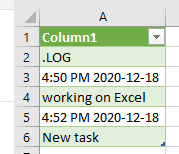
You can leave the default settings and Load the data as is as it’ll likely leave all your text entries in vertical form, which will still work for our purposes. Here’s a sample of what my log file looks like after importing it into Excel:

Text data in Excel.

If you’re using one of the newer versions of Excel that includes PowerQuery, a connection is created when you import the text file into your spreadsheet. This prevents you from having to re-import the file manually each time to check for changes. You only need to refresh the data and it will pull in the changes for you.

And if you make additional entries to your text file, save it, and refresh the data in the spreadsheet and it will update. Just simply right-click on one of the entries in column A, select Refresh, and the data will update from the file — as long as it remains saved in the same place.

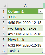
If, after an hour I make another entry to make log file and click on update in the Excel file, the information is up-to-date without having to initiate another import process:

Importing text data into Excel.

This is where Excel is very powerful and effective in making it easy to pull data from another file. However, the data isn’t in a form that’s terribly useful to us in the form that it’s in now. Let’s move on to the next part: setting up the template in Excel so that the time log will be a lot more user friendly.

Creating a template to populate the information correctly

The data is in column A, and what I’ll do is create headers in columns C:F for the Start Time, the Task itself, the End Time, and the Duration (in minutes). Here’s what that looks like:

Creating a log file in Excel.

Now, I’ll need to enter in formulas to populate all those fields. The start time field will initially pull from the third row in column A, and then it will grab every second row after that. So let’s start with building out that logic.

I’ll start with using an INDEX() formula to pull a value from column A. Since there’s only one column I’ll be extracting data from, the key argument is going to be the row number. The third row is where my first entry is, so for the row number I’ll start with the number three. Here’s what my formula looks like thus far:

=INDEX(A:A,3,1)

I select row 3 and column 1. This will only work for the first value. I need to adjust the formula so that it will automatically adjust based on which row I’m on, so that it knows to take either the first time entry, the second, the third, and so on. The ROW() function is helpful in this case because it will return the row number of the current cell. And since my first entry in the table will be on the second row, I’ll want to remove the first two rows. My row calculation looks like this right now:

3+ROW(C2)-2

For the first entry (on the second row), this will evaluate out to 3, since ROW(C2) will equal 2 and it will minus 2 from that. This still works for the first entry, but if I were to copy this formula down it would not give me the correct result for other entries. For instance, in row 3, the formula would be as follows:

3+ROW(C3)-2 this would evaluate to 3+(3)-2 = 4

But row 4 contains my task description, not the next timestamp. I need to double with each row I go down. I need to adjust my formula for the row calculation back in C2 to be as follows:

3+(ROW(C2)-2)*2

Now, the row number minus 2 will then multiply by 2. If I copy this formula down to cell C3, it’ll look as follows:

3+(ROW(C3)-2)*2 : this would evaluate to 3+(3-2)*2 = 3+(1)*2 = 5

This returns row 5, which is the next timestamp in column A. If I copy the formula down to row 4, then it will return the 7th item in the column, which is again the next timestamp. Now that the formula is correctly returning each odd-numbered row, I can use this formula for the template I’ve created. My full formula in column C2 looks as follows:

=INDEX(A:A,3+(ROW(C2)-2)*2,1)

This will work not only for the initial timestamp but it will also extract entries that come after it. All you need to do is copy the formula down.

I can replicate this for the Task field in column D. The only change I need to make is to use row 4 as my starting point rather than 3. And so my formula for the task column looks as follows:

=INDEX(A:A,4+(ROW(C2)-2)*2,1)

For the end time, I’ll use row 5 as my starting point. The end of one task will be the same as the start of the next task. And then all that’s left is to calculate the task duration in column F. The calculate the difference in times, I’ll start by taking the end time and subtracting the start time. However, this will give me a decimal that isn’t very easy to interpret:

Log file in Excel with one row of data.

The reason is that Excel converts this into a fraction of a day. A two-minute interval is less than 1% of the 1,440 minutes that are in each day, which is why the number is so low. To convert the duration into hours I can multiply it by 24, and then the number changes to 0.033, which is the fraction of an hour that two minutes represents. But if I want to go further and convert this into total minutes, I’ll multiply this again by a factor of 60. Now my formula looks as follows:

=(E2-C2)*24*60

Now, after rounding off the decimal points, my duration calculation in column F correctly gives me the number of minutes between the start and end time of a task:

Log file in Excel with calculations.

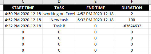
The table is now set up and you can just copy these formulas down to accommodate more entries. You’ll end up with a series of zeroes if there’s not enough data in column A. If you want a cleaner solution, what you can do is use the COUNTA() function to determine the number of rows that are in column A and determine whether to apply a formula or not. For instance, in my example, my data goes until the 8th row and so my formulas look fine for the first two entries but after that, there is no end time for the third task and the subsequent entries are full of zeroes:

Log file in Excel with missing entries.

It’s not a terribly elegant solution at this point. To get around this, I’ll create a rule for each column to say that if there is no entry, it will be blank. For the start time, I’ll add the following to the beginning of the formula:

IF(COUNTA(A:A)<(3+(ROW(C2)-2)*2),””

This will check if there are enough rows in column A to extract a value for the current cell. If not, the value will be blank. Here’s how the full formula looks in cell C2:

=IF(COUNTA(A:A)<(3+(ROW(C2)-2)2),””,INDEX(A:A,3+(ROW(C2)-2)2,1))

For column D, the formula uses row 4 instead of row 3:

=IF(COUNTA(A:A)<(4+(ROW(C2)-2)2),””,INDEX(A:A,4+(ROW(C2)-2)2,1))

And for column E:

=IF(COUNTA(A:A)<(5+(ROW(C2)-2)2),””,INDEX(A:A,5+(ROW(C2)-2)2,1))

For the duration calculation, I will check to make sure there are values in both the start and end time, otherwise, the value will be blank:

=IF(OR(C2=””,E2=””),””,(E2-C2)*24*60)

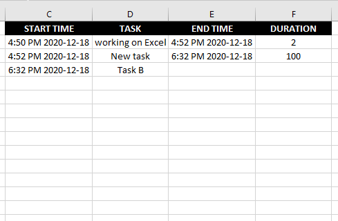
With these formulas now set up, I can copy them down hundreds of rows down if I want and they won’t result in a series of zeroes or errors:

Log file in Excel.

The data in Excel will now auto-populate as I add more entries to the time log and at the same time it won’t be an eyesore if there is incomplete data.


If you liked this post on how to create a time log in Excel, please give this site a like on Facebook and also be sure to check out some of the many templates that we have available for download. You can also follow us on Twitter and YouTube.

linebreak2

How to Make a Line Break in Excel

Are you entering multiple lines of text in Excel and want to break it up into multiple lines? You don’t have to adjust the cell size to do it and below I’ll show you some ways that you can manage cells that contain a lot of text, including how to make a line break in Excel.

Creating a line break

Here’s an example of a cell that could use a line break:

Text bleeding over into another cell.

Currently, this bleeds onto where the start of the next cell should be. But rather than adjusting the length of my cell, I can position my cursor right after the period and before the ‘T’, hit ALT+ENTER, and now my cell looks like this:

Text after applying wrap text.

Please note that if you want to create another line, you can’t just click on the cell and enter ALT+ENTER, you actually need to be inside the cell entering in values. To get into edit mode you can either click into the formula bar with the cell selected or click F2. Then, it’s a matter of selecting where you want to insert the line break. In the above example, the optimal position is just before the start of the second sentence. Then, once you’re there, you’ll click ALT+ENTER to move the following text down a line. You can repeat these steps to create as many lines as you’d like.

When creating an extra line, Excel automatically expands my cell vertically and selects the option to Wrap Text which is on the Home tab:

Wrap Text enabled.

Using the ALT+ENTER shortcut tells Excel that you want to wrap your text and create a new line, which is what I’ve done in this example. Once wrap text is selected, your data will automatically conform to its cell size; the contents won’t bleed over into adjacent cells. For example, if I shrink my cell size then it no longer goes into the next cell, it just simply doesn’t show up:

Wrapped text that is in a cell that isn't wide enough.

If I were to double-click and auto-fit the column, then my cell would expand horizontally to accommodate the contents:

Wrapped text that's long enough horizontally.

However, if I were to double-click on the row and use auto-fit there, then the row would get larger and then my cell looks as follows:

Wrapped text that is expanded vertically rather than horizontally.

As you can see, once you’ve enabled Wrap Text, you don’t have to worry about your cell’s values moving into other cells. But at the same time, you may not necessarily want Wrap Text enabled for every cell since there’s the possibility that text gets cut off.

A good benchmark I normally use, especially for headers and where text may span multiple lines is to set the row height to 30. If that’s not enough, then I would at that point look at expanding the cell horizontally.

Another option that you have at your disposal if you want to accommodate a large value of text is to use Merge Cells. Generally, I’m not a big fan of merging cells because it can be problematic with formulas. But if you’re reserving this primarily for headers and text where there won’t be numbers in or near it, then it could be a practical alternative. That being said, I’d still keep this as a last resort.


If you liked this post on how to make a line break in Excel, please give this site a like on Facebook and also be sure to check out some of the many templates that we have available for download. You can also follow us on Twitter and YouTube.

convertsummary

Convert a Summary Table in Excel Into a Pivot Table

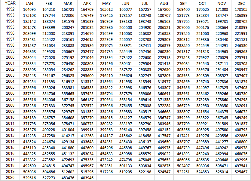
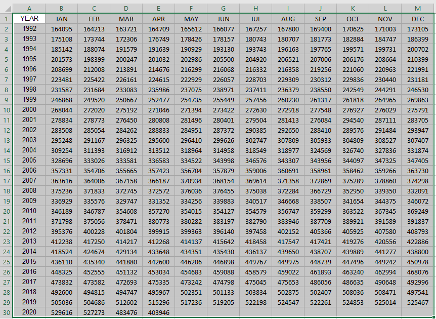
Often times, when you download a data table from somewhere it’s not in the format you need it to be. Tables are often in a summary format where you have months going down and years going across, or vice versa. It’s the end result of what you want a pivot table to look like, but you can’t easily turn that into a pivot table itself. Below, I’ll show you how to turn a summary table in Excel that looks like this:

Summary table.

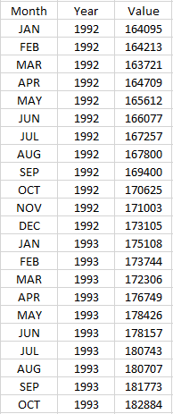
Into this:

Data in tabular format in Excel.

This format is much more Excel-friendly and one that you can easily convert into a pivot table.

Converting the table

The data I’m using is the same one that I used in an earlier post that went over transposing data. Transposing data, unfortunately, isn’t enough to make data workable if you want to convert it into a pivot table. You’ll want data to be in a tabular format so that there’s a header for the month, year, and value.

You could manually transpose one year at a time and copy the data one by one. But of course, that isn’t optimal at all. The good news is I’ve got a macro that can help you flip that data in one click. It will go through the painstaking process of reorganizing the data for you.

Here’s the code for the macro. You can just put it into a module (I’ll leave a template to download below if you aren’t comfortable doing this step yourself):

Sub flipdata()

Dim cl, nxtcl As Range
Dim lastcol, lastrow, firstcol, firstrow As Integer


'get total number of rows and columns in range
lastcol = Selection.End(xlToRight).Column
lastrow = Selection.End(xlDown).Row

'get first column and row
firstcol = Selection.Column
firstrow = Selection.Row

'assign output starting point
Set nxtcl = Cells(lastrow + 2, firstcol)

nxtcl = "Header 1"
nxtcl.Offset(0, 1) = "Header 2"
nxtcl.Offset(0, 2) = "Value"

Set nxtcl = nxtcl.Offset(1, 0)


'cycle through data

For yr = (firstrow + 1) To lastrow

    For mth = (firstcol + 1) To lastcol

        nxtcl = Cells(firstrow, mth)
        nxtcl.Offset(0, 1) = Cells(yr, firstcol)
        nxtcl.Offset(0, 2) = Cells(yr, mth)
        Set nxtcl = nxtcl.Offset(1, 0)

    Next mth

Next yr

End Sub

It will output the data a couple of rows below where your data ends. It’s important to select the entire range of data before running the macro since it will go through the range that you’ve selected, nothing else. And if there’s data below your selection, it will overwrite that.

After you’ve selected the data, then you run the macro. In my template, I’ve got a button that you can press that will do the job for you and then you’ll get something that looks like this:

Data in tabular form.

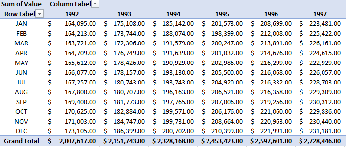
Once in this format, you can easily create a pivot table:

Pivot table.

If you’d like to download the file that contains the macro, it’s available here.


If you liked this post on how to convert a summary table in Excel into a pivot table, please give this site a like on Facebook and also be sure to check out some of the many templates that we have available for download. You can also follow us on Twitter and YouTube.

Man entering data into a computer.

8 Ways to Speed Up Data Entry in Excel

Entering data into Excel isn’t much fun, especially if you’ve got a lot of it to enter. The good news is that there are plenty of ways that you can expedite the process so that it’s more efficient and takes less time. Here are eight ways that you can make data entry in Excel a whole lot quicker:

1. Using tab to cycle through your fields

If you’re entering fields across several columns, using the tab button can make it easier to enter data rather than using the arrow keys. And by hitting the TAB button, once you’re at your last column, you can hit the ENTER key and you’ll start from the beginning of the next line. As long as you keep tabbing over, Excel will remember which column you started from when you press ENTER.

Even if you accidentally tab over one or two fields too many, you still don’t have to use the arrow keys. All you have to do is press SHIFT+TAB and you will move in the opposite direction. It has the reverse effect of just pressing the TAB key. Similarly, the ENTER key will bring you down a row while SHIFT+ENTER will move you up a row.

Anytime you can avoid using the mouse or arrow keys, your data entry in Excel can go a lot quicker.

2. Using CTRL+D and CTRL+R to copy data

If you need to copy data from the cell directly above, you can use the CTRL+D shortcut and it will do just that. And if you want to copy data from the left, then you’ll use CTRL+R. This will work the same as if you were to drag the cells. That means that formulas will copy over as well.

3. Use Page Up and Page Down to cycle through tabs

This is another shortcut that can help you quickly jump through different tabs in your workbook. Page Down will cycle through the worksheets to the right, and Page Up will go through the worksheets that are to the left of your active sheet. If you’re entering a lot of data across many tabs, this will help you avoid having to use the mouse to switch tabs.

4. Entering data in multiple worksheets at once

If you have to enter the same data, the same formula, or if you just need to change the formatting so it’s the same across all worksheets, the good news is you don’t have to do one tab at a time. Instead, select all the sheets that you want to make the changes to and then enter the data or make the changes you need to make in any one of them. If the worksheets are all selected, the changes will be applied to all of them.

Multiple tabs selected in an Excel spreadsheet.

In the above screenshot, I’ve selected Sheet1, Sheet2, Sheet3, and Sheet4. The one I’m currently in is Sheet1. Any changes that I make in that sheet will carry over to the others.

Be careful, however, because if you make a change in cell A1, then A1 will change for all the worksheets that you’ve selected. If your data is structured slightly differently in the sheets, this may give you some unexpected results. This should only be used if your data is in the exact same structure. For formatting, however, it’s an easy way to apply formatting to many sheets at once. But when you’re entering data or formulas, you should double-check which cells you’ll be entering the data into to make sure that they’re correct and won’t cause issues across all the different sheets.

5. Moving quickly throughout your worksheets

Tabbing over can be helpful as you’re entering data, but it may not be of much help if you need to go to the end of your data set. For this, there are a couple of things you can do. If you want to go to the last row of your data, double click on the bottom of your active cell, which will send you to the last row where data is entered in that column. If you want to go to the furthest column to the right, double click on the right border of your current cell selection.

Alternatively, what you can do is use the CTRL key along with the arrow keys. For instance, if you want to go to the last row in the column that you’re in, use CTRL + DOWN. And if you want to go to the furthest column in the row that you’re in, use CTRL + RIGHT.

6. Make sure to freeze panes

When you’re entering data into many different columns, freezing the headers at the top can make it easy to ensure you’re entering the right information in the correct field. You may forget where you are if you’re working on many different fields and by freezing panes, you can ensure you have enough data to look at regardless of how many rows down you, and that can lead to wasted time. If you’re not familiar with freezing panes, this post can help give you a quick overview.

7. Maximize your white space

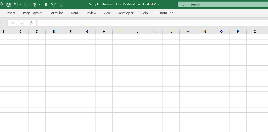
If you’re on a laptop or a small screen or just need to see a lot more data, you can hide some unneeded space in your spreadsheet. That can make it easier to enter data and minimize distractions. For starters, you can minimize the ribbon by double-clicking on any one of the heading names:

Ribbon tabs minimized.

You can still use the ribbon and access it, but this way it gets out of your way unless you actually click on any of the headings again. To undo this, just double-click a header and you’ll get your full-sized ribbon back.

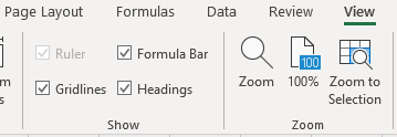
Next up, click on the View tab where you’ll see a few more things you can change:

View settings in Excel.

Here you can uncheck the Formula Bar and even the Headings, assuming you don’t need to see this, of course.

Excel spreadsheet with hidden formula, headings and ribbon minimized.

At this rate, your spreadsheet is looking more like just some plain lined paper. And if you need any more white space, then maybe you’re better off simply investing in a bigger monitor or shrinking your resolution.

8. Use a second window

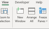
If you have a second monitor, and even if you don’t, you can create a second window within Excel. Whether you’re entering data into multiple different sheets or even if you just want to enter data into multiple areas within the same sheet, a second window can help. This way, you’ll avoid having to jump back and forth. To this, go back to the View tab where you’ll see an option to open a New Window:

Open a new window in Excel using the View tab.

From here, you can move your new window onto another monitor or you can just do a split-screen if you only have one. With Windows 10, you can snap windows to the left or right-side of your monitor, making it easy to see two Excel windows at once.

Got any other tips? Submit yours!

Have any tips of your own that use that improve your data-entry experience in Excel? Feel free to email tips@howtoexcel.net and let us know what you’ve found helpful and if we use it in an updated list, we’ll credit you.


If you liked this post on how to speed up data entry in Excel, please give this site a like on Facebook and also be sure to check out some of the many templates that we have available for download. You can also follow us on Twitter and YouTube.