Are you looking for an easy way to log and track your time in Excel? Below, I’ll show you how you can keep track of the time you spend on tasks without the need for a complicated template or to even open up Excel every time to enter in your time. With a combination of Excel and Notepad, you have all the tools you need to quickly and easily track your time and create a log in Excel.
An easy trick to turn Notepad into a log
To make the process of logging time easy, you probably don’t want to have to open up an Excel spreadsheet each time. There’s an easier way to do so and that’s by using Notepad. Open up a new instance of Notepad and write the following in the first line:
.LOG
Save the file as whatever you want, and then close it. Open it up again and you’ll notice there is now a timestamp when you open the file. Because you entered .LOG at the start of the Notepad file, it will now automatically create a timestamp each and every time that you open the file.
Now, when you’re working on a task, just enter in some text, such as “working on Excel,” click save, and close the file. Now, when you’re switching over to another task or want to say that you’ve finished the task, open up the text file again and enter in a new entry. You probably don’t need to say that you’ve ended a task since the start of a new task would effectively tell you that the previous one is over.
The key thing to remember when you’re logging your tasks in Notepad is that you’ll want to save the file once you’ve made an entry, and then close it out. A good place to store the file might be online or on a shared folder, somewhere that you can access it from any computer and that you can easily update from wherever you are. As you keep adding to the log, you’re essentially creating a database of all your entries.
You can create multiple log files depending on what you’re tracking or you can just keep one big list in a single text file. Either way, once you’ve made some entries, what you can do is now extract that time log in Excel, which brings us to the next step:
Pulling the data into Excel
The text file, while useful, isn’t going to be terribly helpful if you want to easily see the time you’ve spent on a given task. This is where Excel can be incredibly useful. To get the information into Excel, go onto the Data tab and import data using the From Text/CSV button.

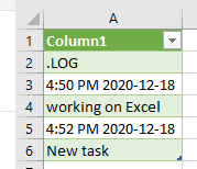
You can leave the default settings and Load the data as is as it’ll likely leave all your text entries in vertical form, which will still work for our purposes. Here’s a sample of what my log file looks like after importing it into Excel:

If you’re using one of the newer versions of Excel that includes PowerQuery, a connection is created when you import the text file into your spreadsheet. This prevents you from having to re-import the file manually each time to check for changes. You only need to refresh the data and it will pull in the changes for you.
And if you make additional entries to your text file, save it, and refresh the data in the spreadsheet and it will update. Just simply right-click on one of the entries in column A, select Refresh, and the data will update from the file — as long as it remains saved in the same place.
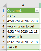
If, after an hour I make another entry to make log file and click on update in the Excel file, the information is up-to-date without having to initiate another import process:

This is where Excel is very powerful and effective in making it easy to pull data from another file. However, the data isn’t in a form that’s terribly useful to us in the form that it’s in now. Let’s move on to the next part: setting up the template in Excel so that the time log will be a lot more user friendly.
Creating a template to populate the information correctly
The data is in column A, and what I’ll do is create headers in columns C:F for the Start Time, the Task itself, the End Time, and the Duration (in minutes). Here’s what that looks like:

Now, I’ll need to enter in formulas to populate all those fields. The start time field will initially pull from the third row in column A, and then it will grab every second row after that. So let’s start with building out that logic.
I’ll start with using an INDEX() formula to pull a value from column A. Since there’s only one column I’ll be extracting data from, the key argument is going to be the row number. The third row is where my first entry is, so for the row number I’ll start with the number three. Here’s what my formula looks like thus far:
=INDEX(A:A,3,1)
I select row 3 and column 1. This will only work for the first value. I need to adjust the formula so that it will automatically adjust based on which row I’m on, so that it knows to take either the first time entry, the second, the third, and so on. The ROW() function is helpful in this case because it will return the row number of the current cell. And since my first entry in the table will be on the second row, I’ll want to remove the first two rows. My row calculation looks like this right now:
3+ROW(C2)-2
For the first entry (on the second row), this will evaluate out to 3, since ROW(C2) will equal 2 and it will minus 2 from that. This still works for the first entry, but if I were to copy this formula down it would not give me the correct result for other entries. For instance, in row 3, the formula would be as follows:
3+ROW(C3)-2 this would evaluate to 3+(3)-2 = 4
But row 4 contains my task description, not the next timestamp. I need to double with each row I go down. I need to adjust my formula for the row calculation back in C2 to be as follows:
3+(ROW(C2)-2)*2
Now, the row number minus 2 will then multiply by 2. If I copy this formula down to cell C3, it’ll look as follows:
3+(ROW(C3)-2)*2 : this would evaluate to 3+(3-2)*2 = 3+(1)*2 = 5
This returns row 5, which is the next timestamp in column A. If I copy the formula down to row 4, then it will return the 7th item in the column, which is again the next timestamp. Now that the formula is correctly returning each odd-numbered row, I can use this formula for the template I’ve created. My full formula in column C2 looks as follows:
=INDEX(A:A,3+(ROW(C2)-2)*2,1)
This will work not only for the initial timestamp but it will also extract entries that come after it. All you need to do is copy the formula down.
I can replicate this for the Task field in column D. The only change I need to make is to use row 4 as my starting point rather than 3. And so my formula for the task column looks as follows:
=INDEX(A:A,4+(ROW(C2)-2)*2,1)
For the end time, I’ll use row 5 as my starting point. The end of one task will be the same as the start of the next task. And then all that’s left is to calculate the task duration in column F. The calculate the difference in times, I’ll start by taking the end time and subtracting the start time. However, this will give me a decimal that isn’t very easy to interpret:

The reason is that Excel converts this into a fraction of a day. A two-minute interval is less than 1% of the 1,440 minutes that are in each day, which is why the number is so low. To convert the duration into hours I can multiply it by 24, and then the number changes to 0.033, which is the fraction of an hour that two minutes represents. But if I want to go further and convert this into total minutes, I’ll multiply this again by a factor of 60. Now my formula looks as follows:
=(E2-C2)*24*60
Now, after rounding off the decimal points, my duration calculation in column F correctly gives me the number of minutes between the start and end time of a task:

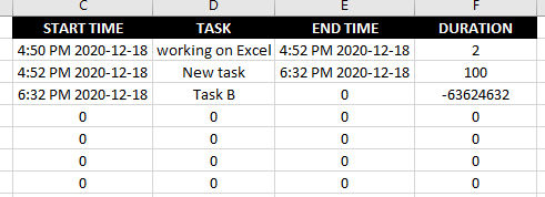
The table is now set up and you can just copy these formulas down to accommodate more entries. You’ll end up with a series of zeroes if there’s not enough data in column A. If you want a cleaner solution, what you can do is use the COUNTA() function to determine the number of rows that are in column A and determine whether to apply a formula or not. For instance, in my example, my data goes until the 8th row and so my formulas look fine for the first two entries but after that, there is no end time for the third task and the subsequent entries are full of zeroes:

It’s not a terribly elegant solution at this point. To get around this, I’ll create a rule for each column to say that if there is no entry, it will be blank. For the start time, I’ll add the following to the beginning of the formula:
IF(COUNTA(A:A)<(3+(ROW(C2)-2)*2),””
This will check if there are enough rows in column A to extract a value for the current cell. If not, the value will be blank. Here’s how the full formula looks in cell C2:
=IF(COUNTA(A:A)<(3+(ROW(C2)-2)2),””,INDEX(A:A,3+(ROW(C2)-2)2,1))
For column D, the formula uses row 4 instead of row 3:
=IF(COUNTA(A:A)<(4+(ROW(C2)-2)2),””,INDEX(A:A,4+(ROW(C2)-2)2,1))
And for column E:
=IF(COUNTA(A:A)<(5+(ROW(C2)-2)2),””,INDEX(A:A,5+(ROW(C2)-2)2,1))
For the duration calculation, I will check to make sure there are values in both the start and end time, otherwise, the value will be blank:
=IF(OR(C2=””,E2=””),””,(E2-C2)*24*60)
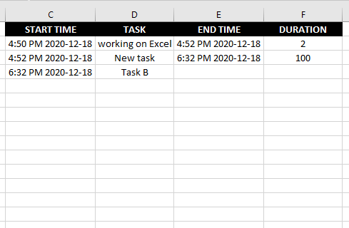
With these formulas now set up, I can copy them down hundreds of rows down if I want and they won’t result in a series of zeroes or errors:

The data in Excel will now auto-populate as I add more entries to the time log and at the same time it won’t be an eyesore if there is incomplete data.
If you liked this post on how to create a time log in Excel, please give this site a like on Facebook and also be sure to check out some of the many templates that we have available for download. You can also follow us on Twitter and YouTube.

