8 Ways to Speed Up Data Entry in Excel

Entering data into Excel isn’t much fun, especially if you’ve got a lot of it to enter. The good news is that there are plenty of ways that you can expedite the process so that it’s more efficient and takes less time. Here are eight ways that you can make data entry in Excel a whole lot quicker:

1. Using tab to cycle through your fields

If you’re entering fields across several columns, using the tab button can make it easier to enter data rather than using the arrow keys. And by hitting the TAB button, once you’re at your last column, you can hit the ENTER key and you’ll start from the beginning of the next line. As long as you keep tabbing over, Excel will remember which column you started from when you press ENTER.

Even if you accidentally tab over one or two fields too many, you still don’t have to use the arrow keys. All you have to do is press SHIFT+TAB and you will move in the opposite direction. It has the reverse effect of just pressing the TAB key. Similarly, the ENTER key will bring you down a row while SHIFT+ENTER will move you up a row.

Anytime you can avoid using the mouse or arrow keys, your data entry in Excel can go a lot quicker.

2. Using CTRL+D and CTRL+R to copy data

If you need to copy data from the cell directly above, you can use the CTRL+D shortcut and it will do just that. And if you want to copy data from the left, then you’ll use CTRL+R. This will work the same as if you were to drag the cells. That means that formulas will copy over as well.

3. Use Page Up and Page Down to cycle through tabs

This is another shortcut that can help you quickly jump through different tabs in your workbook. Page Down will cycle through the worksheets to the right, and Page Up will go through the worksheets that are to the left of your active sheet. If you’re entering a lot of data across many tabs, this will help you avoid having to use the mouse to switch tabs.

4. Entering data in multiple worksheets at once

If you have to enter the same data, the same formula, or if you just need to change the formatting so it’s the same across all worksheets, the good news is you don’t have to do one tab at a time. Instead, select all the sheets that you want to make the changes to and then enter the data or make the changes you need to make in any one of them. If the worksheets are all selected, the changes will be applied to all of them.

In the above screenshot, I’ve selected Sheet1, Sheet2, Sheet3, and Sheet4. The one I’m currently in is Sheet1. Any changes that I make in that sheet will carry over to the others.

Be careful, however, because if you make a change in cell A1, then A1 will change for all the worksheets that you’ve selected. If your data is structured slightly differently in the sheets, this may give you some unexpected results. This should only be used if your data is in the exact same structure. For formatting, however, it’s an easy way to apply formatting to many sheets at once. But when you’re entering data or formulas, you should double-check which cells you’ll be entering the data into to make sure that they’re correct and won’t cause issues across all the different sheets.

5. Moving quickly throughout your worksheets

Tabbing over can be helpful as you’re entering data, but it may not be of much help if you need to go to the end of your data set. For this, there are a couple of things you can do. If you want to go to the last row of your data, double click on the bottom of your active cell, which will send you to the last row where data is entered in that column. If you want to go to the furthest column to the right, double click on the right border of your current cell selection.

Alternatively, what you can do is use the CTRL key along with the arrow keys. For instance, if you want to go to the last row in the column that you’re in, use CTRL + DOWN. And if you want to go to the furthest column in the row that you’re in, use CTRL + RIGHT.

6. Make sure to freeze panes

When you’re entering data into many different columns, freezing the headers at the top can make it easy to ensure you’re entering the right information in the correct field. You may forget where you are if you’re working on many different fields and by freezing panes, you can ensure you have enough data to look at regardless of how many rows down you, and that can lead to wasted time. If you’re not familiar with freezing panes, this post can help give you a quick overview.

7. Maximize your white space

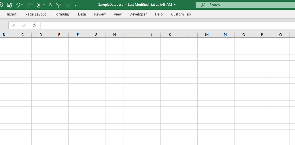
If you’re on a laptop or a small screen or just need to see a lot more data, you can hide some unneeded space in your spreadsheet. That can make it easier to enter data and minimize distractions. For starters, you can minimize the ribbon by double-clicking on any one of the heading names:

You can still use the ribbon and access it, but this way it gets out of your way unless you actually click on any of the headings again. To undo this, just double-click a header and you’ll get your full-sized ribbon back.

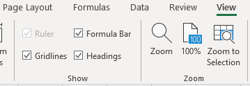
Next up, click on the View tab where you’ll see a few more things you can change:

Here you can uncheck the Formula Bar and even the Headings, assuming you don’t need to see this, of course.

At this rate, your spreadsheet is looking more like just some plain lined paper. And if you need any more white space, then maybe you’re better off simply investing in a bigger monitor or shrinking your resolution.

8. Use a second window

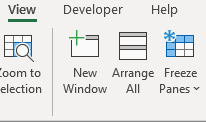
If you have a second monitor, and even if you don’t, you can create a second window within Excel. Whether you’re entering data into multiple different sheets or even if you just want to enter data into multiple areas within the same sheet, a second window can help. This way, you’ll avoid having to jump back and forth. To this, go back to the View tab where you’ll see an option to open a New Window:

From here, you can move your new window onto another monitor or you can just do a split-screen if you only have one. With Windows 10, you can snap windows to the left or right-side of your monitor, making it easy to see two Excel windows at once.

Got any other tips? Submit yours!

Have any tips of your own that use that improve your data-entry experience in Excel? Feel free to email [email protected] and let us know what you’ve found helpful and if we use it in an updated list, we’ll credit you.

If you liked this post on how to speed up data entry in Excel, please give this site a like on Facebook and also be sure to check out some of the many templates that we have available for download. You can also follow us on Twitter and YouTube.