How to Freeze Panes

Freezing panes in Excel is useful when you want to still see certain rows or columns as you scroll through a large data set. Without doing so you could easily get lost in your data trying to figure out which header or category the value you are looking at belongs to.

Under the View tab select Freeze Panes and if panes are frozen you will see an option to unfreeze panes. Otherwise you can choose to select to freeze panes, freeze top row, or freeze first column. Freeze top row will ensure that row 1 is frozen is you scroll down and ensure you will see your headers. Freezing the first column will make sure column A is always visible as you scroll to the right.

Now but what if you wanted to freeze both rows and columns, or multiple rows or multiple columns? That is where you would just use the regular Freeze Panes option. The key here is to select the correct point of intersection. When you press freeze panes the active cell will determine which rows and columns are frozen. Any rows above and columns to the left of the active cell will be frozen.

For example, if you wanted to freeze just the first row, you would select cell A2. Since there is nothing to the left of it, it would only freeze row 1 which is above.

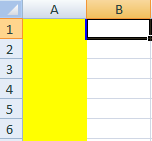
If you wanted to freeze just column A, you would select cell B1. Since nothing is above row 1, only column A is to the left of B, so only A would be frozen.

See above for the highlighted column and what cell I would need to select to freeze it.

 If you wanted to freeze column A and row 1 then you would need to select cell B2 since row 1 is above that cell and column A is to the left. See below:

Similarly, if you wanted to freeze the first two columns and the first two rows you would select cell C3 – see below for results