How to Transpose Data in Excel

It’s not often that you’ll need to transpose data in Excel, but when you do you’ll be happy to know how easy it is to do. In this post, I’ll go over not just transposing data but converting text to columns and showing you how you can change a block of text into data that you can use for analysis. After all, there’s no use trying to transpose data if it isn’t in a workable format.

If you want to follow along, the data I’m going to be using comes from the United States Census Bureau. In particular, I’ll be pulling the monthly retail and food services sales data for the past couple of decades. You can download that information here.

Copying the data into excel

Let’s start with the first step, and that’s to get the data into Excel. It’s in text, but the information is workable since it’s in the format of a table. I’m not going to copy the seasonal factors, I just want the raw, unadjusted sales numbers. To get the data into Excel, I’ll just highlight the sales data, copy it, and then paste it into a blank Excel sheet. Here’s how it looks:

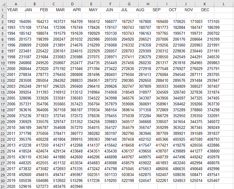
The first thing that needs to be fixed is that everything is in column A. The data as it is won’t be useful for data analysis and needs to be cleaned up before it would make sense to try and transpose it.

Use text to columns to spread data across multiple columns

In Excel, there’s a Text to Columns button right on the Data tab that will help you to quickly and easily spread the data onto many columns. In our example, select column A and click on this button or something that looks similar to it if you’ve got an older version of Excel:

You’ll then see an option for how you want to break out the data. The default is Fixed Width:

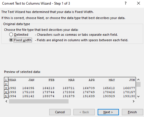
However, that’s not an ideal way to split the data and it rarely ever is. Unless the data is always the same length it won’t be very useful. At best, it’ll be time-consuming to get the output in the format that you’re after. Instead, change the option to Delimited. Click on Next, and then you’ll see various options for splitting the data:

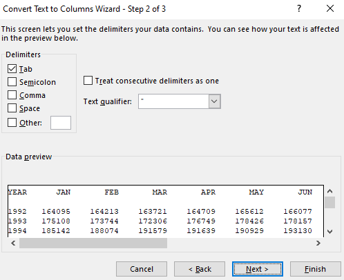
The data isn’t separated by a semicolon, comma, or any other distinctive character. There is, however, a space between each amount. That’s why we’ll want to unselect Tab and tick off the box for Space instead. We see a preview of how the data will be separated, which looks to be what we’re after:

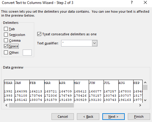
At this point we can just click the Finish button and our output will now look like this:

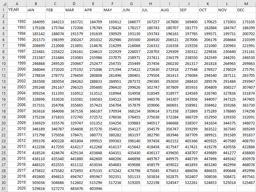
Now we’ve got data that’s much more usable as every number is in its own individual cell. The one thing we’ll want to do before we get to transposing it is to get rid of row 2. The blank row effectively separates the headers from the data, and that’s not ideal.

Next up, let’s get to the actual transposing part.

Transposing the excel data

By transposing data, you’re flipping the rows and columns around. And to do that is pretty straightforward. First, copy the data, including the headers, and then click on a blank cell — I’m going to pick O1. Then, right-click and select Paste Special. There, you’ll see an option at the bottom that says Transpose:

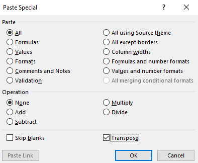
Then your data will be flipped, or transposed. You can also select Transpose right from the Paste Special menu and select the icon from there. You can also use shortcut keys S and T to select the menu and then select the transpose button.

Now the data looks like this:

The years are now spread across the columns while the months are going down the rows.

Ultimately, whichever way you want to see the data comes down to personal preference. And by transposing it, you can change the view easily to make that happen.

If you liked this post on how to make a transpose data in Excel, please give this site a like on Facebook and also be sure to check out some of the many templates that we have available for download. You can also follow us on Twitter and YouTube.