FixNAErrors

How to Fix #N/A Errors in Excel

Excel is a powerful tool, but even the most experienced users encounter errors like #N/A from time to time. This error can be frustrating, but it’s actually Excel’s way of saying it can’t find the information it’s looking for. Let’s break down why this error happens, and how to fix it.

What does #N/A mean?

The #N/A error occurs when a formula cannot find a value it’s supposed to look up. This commonly happens with lookup functions like VLOOKUP, HLOOKUP, INDEX and MATCH, or XLOOKUP.

Common Reasons for #N/A Errors

When a value isn’t found in your lookup formula, there are multiple possible reasons why that might happen. Here are some of the most common issues:

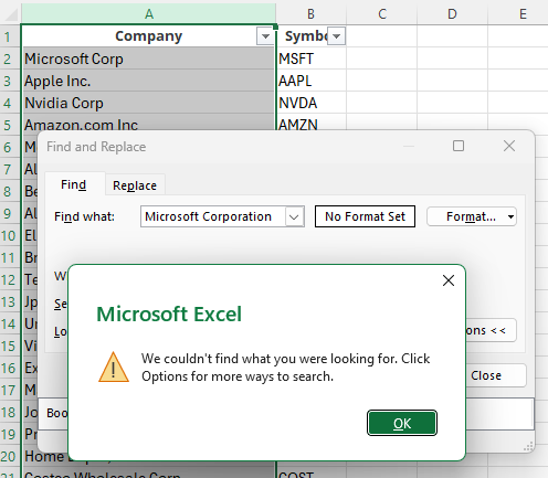
The value isn’t in the lookup range. The simplest reason is that the value simply isn’t there. Perhaps the value you’re looking for is spelled differently than what you’re searching for, or it just isn’t contained within the data set. An easy way to check for this is to use the CTRL+F shortcut and manually search for the value. If it isn’t found, you’ll get a message saying the value isn’t found. If it is, then it’s likely one of the other reasons that’s causing the error.

An error stating that a value isn't found within a range.

In the above error, ‘Microsoft Corporation’ isn’t found because the text in the range is just ‘Microsoft Corp’

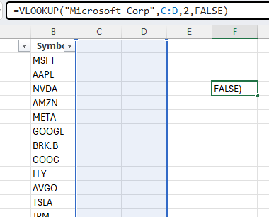
The range or table being searched is incorrect. In this situation, your value exists but it can be that you’re looking in the wrong place. For example, if your data set is in columns A:B but you’re looking at values in C:D, then the value won’t be found. The only way to catch this is to manually look at your formula. By clicking into the formula, it will highlight the range it’s looking at. If it doesn’t look like you’ve selected the right area, that can explain why you are encountering an error.

A VLOOKUP formula which is searching in the incorrect range.

The data types are not the same. In this situation, you may be searching for a numerical value of 1 but the actual value is a text value of 1. This can be a more challenging issue to uncover. However, by using the CTRL+F function you can confirm if the value is indeed found. And if it is found, what you can do is use a formula to check if the values are an exact match. Suppose your lookup value is in cell A1 and the matching value is in cell D100. You can enter the following formula below, to confirm whether it is an exact match:

=A1=D100

If there is an error, that means the data is not the same. At this stage, you may want to do a closer analysis of the values to see if there are any extra characters. You may also want to use the ISNUMBER function to check whether one value is reading as a number and the other as text, as that could be resulting in the #N/A error as well.

The ISNUMBER function in Excel.

If the result of the ISNUMBER formula is FALSE, that tells us that the value is not a number despite it appearing to be.

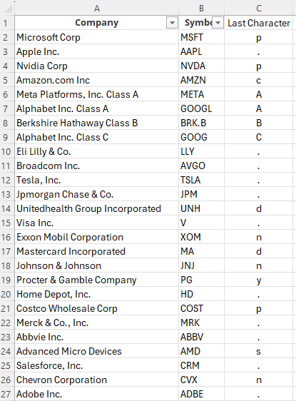
There are trailing spaces. If your data type is the same and it looks like everything should be matching, then it may be an issue that you have a trailing space, either in your lookup value or the value which it should be matching to. An easy way to check for trailing spaces is by using the RIGHT function. If you don’t specify the number of characters you want to extract from the right, it will by default grab the last one. Then, if you see the formula returning characters, you know there are no trailing spaces. If, however, there is a blank value, this would be confirmation that a blank space exists at the end, and it could be interfering with your lookup.

Checking the last character in a range of cells.

In the above example, column C shows the last character. While there are letters and punctuation, there are no blank values shown.

How to use formulas to suppress #N/A errors

If all else fails and you can’t find the reason for the #N/A error, or it’s not possible to eliminate it without drastically changing your spreadsheet, or you simply don’t have the time to look through all the possible reasons, then you can use formulas to suppress the errors for the sake of eliminating them. There are two options here.

IFNA

The IFNA function can replace the error value with a different value of your choosing. You may want to simply have an empty value, perhaps a 0, or just a different message altogether. In the following formula, I’m using the IFNA function to return a text value of “Not Found” if the value in F4 is not found within column A:

=IFNA(VLOOKUP(F4,A:B,2,FALSE),”Not Found”)

If you encounter any other error, then you’ll still see an error. This function will only suppress #N/A errors.

IFERROR

The IFERROR function works similarly to the IFNA function but the key difference is it will suppress any and all errors. You can deploy it in the same way as you would the formula above:

=IFERROR(VLOOKUP(F4,A:B,2,FALSE),”Not Found”)

The advantage of using this function is it will remove any errors. But that can also be a drawback because if there are different issue causing the error, it won’t be evident, and that can mask other problems within the spreadsheet.


If you like this post on How to Fix #N/A Errors in Excel, please give this site a like on Facebook and also be sure to check out some of the many templates that we have available for download. You can also follow me on Twitter and YouTube. Also, please consider buying me a coffee if you find my website helpful and would like to support it.

GetRidofWarning6

How to Get Rid of the Red Warning Bar in Microsoft Excel

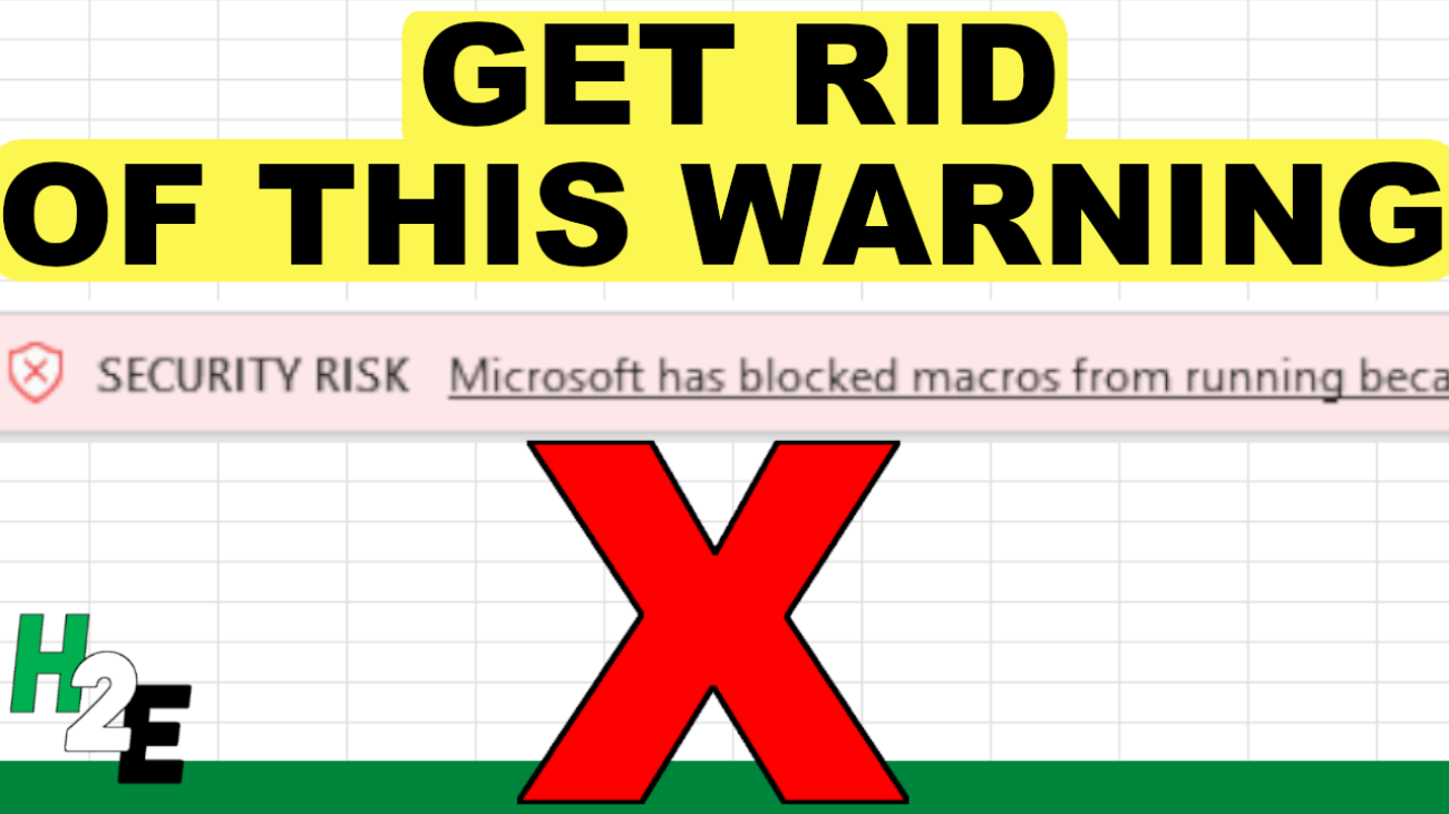
Have you opened a file in Excel which contains macros in it only to find that you can’t use it, because the content is blocked? If you’ve come across the following warning bar, I’m going to show you how can you remove it once and for all.

Red warning bar in Microsoft Excel.

This is different than the yellow warning bar in the past where you can just click on Enable Content and be on your way. This fix requires an extra step.

Here’s how to get rid of the red warning bar

1. Close out of the Excel file completely.

2. Right-click on the file and select properties.

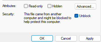
3. In the file properties, check off the option to Unblock the file and then click Apply.

4. Re-open the file, where you’ll be back to seeing the more familiar, yellow warning bar where you can select to Enable Content.

Once you click on that button, your file will now be able to run macros.

How can you prevent the red warning bar from popping up in Excel?

If you’re running Windows 11 then every Excel file that you download from the internet will have the red warning bar by default. Even if you send the file to yourself and open it from Outlook, you’ll see that error come up. There is, however, a way to get around it.

Here’s what you can to avoid encountering the red warning bar on macro-enabled Excel files:

  1. In Excel, go to File -> Options
  2. Go to the Trust Center and select Trust Center Settings
  3. Navigate to Trusted Locations
  4. Click on the button to Add new location
  5. Input a location on your computer where you plan to save macro-enabled files and click OK. You can select the option to include subfolders as well.

Any file you save in one of your trusted locations won’t get the red warning bar anymore — you’ll still have the yellow warning bar, however, depending on your macro security settings. But you’ll now able to enable content without having to close and re-open the file.


If you like this post on How to Get Rid of the Red Warning Bar in Microsoft Excel, please give this site a like on Facebook and also be sure to check out some of the many templates that we have available for download. You can also follow me on Twitter and YouTube. Also, please consider buying me a coffee if you find my website helpful and would like to support it.

value error

How to Fix #VALUE! Errors in Excel

Microsoft Excel is a powerful tool for data analysis and financial modeling, but encountering errors like #VALUE! can be a frustrating hurdle for many users. This error generally signals an issue with the way your formulas are set up or how data is entered. Understanding the root causes of the #VALUE! error and learning how to fix it can save you time and stress. This article will explore why the #VALUE! error occurs and provide practical solutions to address it.

What Causes the #VALUE! Error?

The #VALUE! error appears in Excel when a formula contains cells that have incompatible data types or when the formula is improperly structured. Here are some common scenarios:

  1. Incorrect Data Types: This is the most frequent cause. Excel expects a certain type of data to perform calculations, but if it receives something different, it will return a #VALUE! error. For example, attempting to multiply a number by a text string will cause this error.
  2. Formula Errors: Sometimes, the error occurs because the formula is not written correctly. For instance, an extra space or a missing operator can lead to #VALUE!.
  3. Cell References: If your formula references a cell that does not contain data or contains inappropriate data (like text in a sum function), Excel will not be able to execute the calculation, resulting in a #VALUE! error.
  4. Date and Time Issues: Excel handles dates and times as serial numbers. Errors can arise when you try to perform operations on what appears to be a date or time but is actually a text string.

How to Fix the #VALUE! Error

Fixing the #VALUE! error involves checking the formula and the data types involved in the computation. Here are some steps you can take:

  1. Check Data Types: Ensure that all data used in calculations are of the correct type. Convert text to numbers if necessary by using Excel functions such as VALUE() or NUMBERVALUE().
  2. Review Formulas: Look for common mistakes like misplaced brackets, incorrect operators, or syntax errors. Excel’s formula auditing tools, found under the “Formulas” tab, can help identify and correct these issues.
  3. Clear Formats: Sometimes, cell formatting can cause issues. Clear all formatting to rule out any hidden formatting errors that might be causing the #VALUE! error.
  4. Use Error Checking: Excel has built-in error checking that can diagnose and offer fixes for various errors, including #VALUE!. This can be accessed from the “Formulas” tab, under “Formula Auditing”.
  5. Simplify Formulas: If your formula is complex, break it down into smaller parts and check each segment individually. This can help isolate the part of the formula that is causing the error.

How to Find the #VALUE! Error

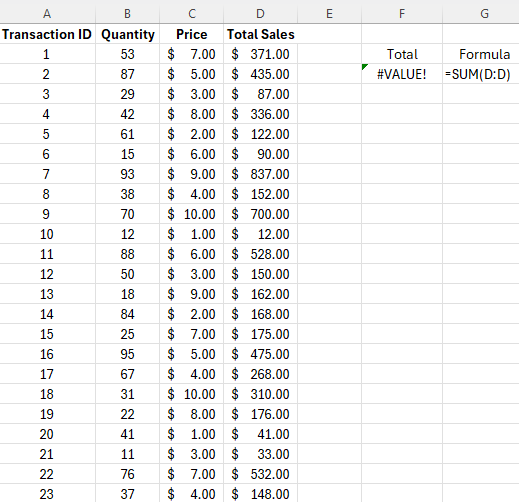
In some cases, it can be difficult to locate the error. In the following example, the formula is summing up column D. But even just a single #VALUE! error within that range will be sufficient to trigger an error in a formula which is just doing a single summation. That’s because you can’t sum up values if they contain the error.

An excel table which contains a #VALUE! error.

The easiest way to find an error within the range is to do the following:

  1. Highlight the range you are checking an error for.
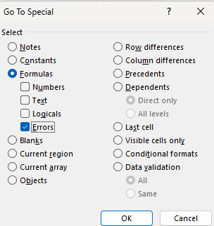
  2. Press F5 and select Special
  3. Select Formulas and uncheck everything except for Errors
Using the go to special menu to find errors in Excel.

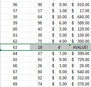
After clicking OK, you will be taken to the first error cell within the range:

A range in Excel which contains a #VALUE! error.

In the highlighted cells, we see that there is an apostrophe after the 4, which turns the value into a text. To correct this, all that’s necessary is to remove the apostrophe. This will fix the calculation as Excel will now recognize the cell as a number; the formula will no longer by trying to multiply a text value against a number, and thus, no error will be present.

Repeat the steps for finding errors until you get the following message:

Best Practices to Avoid Future Errors

To prevent the recurrence of the #VALUE! error, consider the following best practices:

  • Data Validation: Use Excel’s data validation tools to ensure that the correct data types are entered into cells.
  • Template Use: Develop templates with predefined formulas and formatting to minimize the risk of errors.
  • Continuous Learning: Stay updated with Excel’s functionalities and best practices. Regular practice can help you understand and avoid common pitfalls in Excel.

The #VALUE! error in Excel typically stems from data type mismatches or formula mistakes. By carefully checking your data and formulas, and using Excel’s helpful diagnostic tools, you can efficiently resolve these errors and ensure smoother, more accurate data processing in your spreadsheets.


If you like this post on How to Fix #VALUE! Errors in Excel, please give this site a like on Facebook and also be sure to check out some of the many templates that we have available for download. You can also follow me on Twitter and YouTube. Also, please consider buying me a coffee if you find my website helpful and would like to support it.

H2EVlookupWrong

7 Reasons Why VLOOKUP Cannot Find the Right Value

A VLOOKUP function is simple: you enter criteria and select a range that it should extract values from. However, there are multiple reasons why your VLOOKUP cannot find the correct value. Below are seven common reasons your formula may not be working as you expect it to.

In this example, I’m going to use the following list of automobile makes and models:

List of car makes and models.

I’m going to use a lookup formula to find a model and identify the make. The model and make values are in columns A and B on my sheet, respectively. And my lookup value is cell D2. The correct formula would be as follows:

=VLOOKUP(D2,A:B,2,false)

There are four arguments, and here are some of the common ways you could mess this formula up:

1. You didn’t enter the correct range

=VLOOKUP(D2,A1:B100,2,false)

A common error is that you enter a range that doesn’t cover the area that you need. For example, in the above example, the formula goes only to row 100. But if the value you want is on row 101, the lookup formula won’t work and you’ll get an #N/A error.

Another issue could be the following:

=VLOOKUP(D2,B:C,2,false)

In this situation, the formula is starting at column B but the model list is in column A. That all but guarantees that it won’t find the right value. In a VLOOKUP formula, you are looking up the leftmost column in your range. If the model values are in column A, that’s where the formula needs to start from. In the above formula, it will be looking for the values in column B, which isn’t correct.

2. You are extracting values from the wrong column

=VLOOKUP(D2,A:B,3,false)

The range is fixed in this situation but the problem here is that you’re looking for the value in the third column. There are only two that are in the formula. In this instance, you’ll get an error because you’re trying to access a value that’s outside of the range you provided.

=VLOOKUP(D2,A:B,1,false)

The range is correct but here the problem is now you’re referencing the first column. Although you’ll get a value, it will be the same one you input, since the formula is looking at column 1.

One of the common issues with lookup formulas is that people are referencing column numbers that can change over time as they expand their data set. Those numbers won’t automatically adjust when you insert new columns.

There are a couple of workarounds for this. One is to use convert your data set to a table and reference an actual table column. Another is to use the MATCH function to find the column number that you’re looking for. Alternatively, you could use a combination of INDEX & MATCH.

3. You misspelled the value you’re looking up

One of the easier mistakes to spot is when you’ve misspelled the name of what you’re looking up. If in your lookup formula you want to find “Accord” but instead type in “Accorrd” then you’ll end up with another #N/A error. However, if you have a data set where the lookup values could be similar, the danger there is that you could potentially not get an error and instead return the value that relates to a different lookup value. The best way around this is to avoid hardcoding your lookup values. That way, it can be easier to spot errors and it’ll be easier to adjust them.

The reverse is also a problem: if your lookup column contains a misspelling. In that situation, even though the value you’ve looked up is spelled correctly, your lookup could still fail.

4. Your value has extra spaces

One of the trickiest mistakes is where your data isn’t misspelled but contains an extra space somewhere. Just by looking at a cell, you may be able to spot when there’s a leading space. But if there’s a trailing space, that’s tougher and you may not notice until you actually go in and try to edit the value. Whether it’s an extra space or the value is misspelled, that can impact your ability to find a match.

The way to check your data is by using the RIGHT function (or the LEFT function if you want to confirm the first character). If you enter the following formula to reference D2 (the lookup value), it will return the last character in the cell:

=RIGHT(D2)

If it returns a blank value, you’ve found your problem. Similarly, you can use this formula on your lookup list to see if any values have extra spaces. This is something you’ll want to do before creating your lookup formula. Making sure your data is good to go and clean with no trailing spaces can save you from encountering these issues later on.

Removing blank spaces can be easy but sometimes it can be tricky as not all blank values are the same.

5. Your value is reading as the wrong data type

In this example, the lookup is a text value. However, one potential error happens when you’re looking up a number that is stored as text. That can also result in no match being found. A good way to spot this error is to see if your data aligns to the left or the right by default. If you have no formatting applied, text should align to the left, while numbers will shift to the right. Another way you can check if something is reading as text or a number is to use the ISTEXT function. To convert a number stored as text into a number, multiply it by 1.

6. You search for an approximate match when you want an exact match

In most cases, you’ll probably want an exact match from your lookup formula (i.e. you’ll set the last argument to FALSE). The one exception I’ve found to be most useful is when you’re dealing with numbers and ranges. With tax brackets, for example, you’d be looking to see what range a value falls into versus an exact match.

In error #1 on this list, if you set the last argument to TRUE and looked for an approximate match, you would get a result, it just may not be the one you were hoping for.

7. You’ve sorted your formulas and they’re not correct anymore

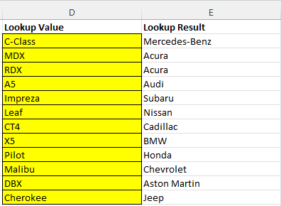
A frustrating problem can be when you’ve entered your formula correctly but when you sort your formulas, they’re now referencing the wrong cells. In this case, you’re dealing with multiple lookups at a time. For example:

Multiple vlookup formulas.

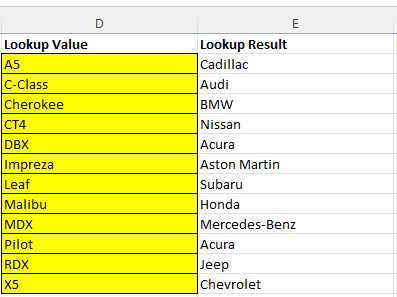
The lookup values are correct but if they get re-sorted, they’re now referencing the wrong values and the lookup results are incorrect:

Lookup values are incorrect after sorting.

After sorting column D in ascending order, the formula is incorrectly saying that Acura makes the Pilot and that there’s a BMW Cherokee. Here’s what the formula looks like in cell E2 before sorting:

=VLOOKUP(Sheet1!D2,A:B,2,FALSE)

The error is in the sheet reference. Since it’s including Sheet1!D2 instead of just D2, the value isn’t automatically updating when resorting. Excel automatically inserts the sheet referencing if you’re editing a formula and jumping from one sheet to another. The formula is locking that value in place, even when you sort. Getting rid of the sheet references fixes the error.


If you liked this post on 7 Reasons Why VLOOKUP Cannot Find the Right Value, please give this site a like on Facebook and also be sure to check out some of the many templates that we have available for download. You can also follow us on Twitter and YouTube.
H2Eerror1

Deleting a Formula in Excel? Do This First

When you’re dealing with complex spreadsheets in Excel, it can sometimes be difficult to tell which cells are safe to delete and which ones you need to keep to ensure everything is working properly. Even cells that look empty could contain formulas. And deleting them can cause problems and wreak your spreadsheet. Before you delete a formula, there’s one thing you can do to prevent that mistake:

Check for dependent cells

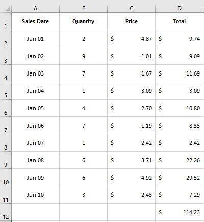
If you’re not sure if a cell is okay to delete and if it has any other cells that depend on it, you can check for dependents. Before deleting a cell, you can click on CTRL + ] which will highlight any cells that use the active cell in a formula (on the current sheet). Here’s a sample spreadsheet that lists price, quantity, and multiples them to get to a total price:

Spreadsheet that calculates the total by multiplying price by quantity.

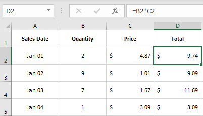
The formula in column D multiples the value in B by C. So that means the value in D depends on the values in C and B (the exception is the subtotal, which depends on the values above it). If I select cell C2 and click on CTRL+], it takes me to cell D2:

The dependent cell is highlighted.

If there is more than one cell that depends on the active cell, then Excel will highlight all of them.

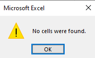
What if there aren’t any dependent cells? In that case, you’ll get the following message:

Message box saying no cells were found.

If you get this message, that means you’re safe to delete the current cell as nothing in the current sheet links to it. However, the one limitation of using the shortcut is that it may not be easy to see all the cells that depend on that one cell. It also won’t tell you if there is a cell on another sheet that uses it.

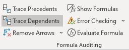
What you can do is use the Trace Dependents button in Excel, which is on the Formulas tab:

Trace Dependents button.

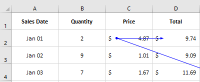
By clicking on this button, arrows will now show up telling me exactly where the dependent cells are:

Arrow showing the dependent cell.

In this situation, the arrow clearly shows an arrow pointing to cell D2. Let’s say I also use the cell in a formula in some place far off in a the same sheet:

Arrows showing multiple dependent cells.

Another line will point to the other cell. If you have a large data model that goes on for many rows and columns, it may not be obvious where the dependent cells are if you use the shortcut key. Using the shortcut can be helpful as a quick check but if you actually want to see all the cells that use the active cell, you’re better off clicking the Trace Dependents button.

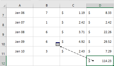
Next, let’s go to the subtotal. Here, let’s assume I’m using this total somewhere on another sheet. Using CTRL+] won’t help me much in this case as it will tell me no cells were found (assuming no cells on the current sheet link to it). But if I click on Trace Dependents, it will show that there is a dependent cell on another sheet:

Dependent cell is on another sheet.

If you double-click on the dotted line (the portion that’s within the cell), the following box will pop up:

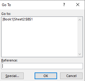
Go to box showing where the dependent cell is located.

This tells us that there is a dependent cell on Sheet2, cell B1. I can go there manually or I can click on the selection and then press OK. Then it will take me directly to the cell:

Dependent cell that links to another sheet.

This isn’t practical on a wide scale as you would have to go one by one and you could have arrows going all over the place. But if you’re not sure about a certain cell, using the Trace Dependents button can be a quick way to see if it’s safe to delete the cell.


If you liked this post on 1 mistake to avoid when deleting formulas in Excel please give this site a like on Facebook and also be sure to check out some of the many templates that we have available for download. You can also follow us on Twitter and YouTube.
circularreference

How to Find Circular References in Excel

If you’re getting an error message in your Excel spreadsheet that there’s a circular reference, that means that at least one of your calculations is referencing back to itself in one way or another. It doesn’t always have to be that two cells are referencing one another. Even indirectly referencing back to a cell can cause a circular reference error.

First thing’s first though, you have to find out where your circular references are before you can fix them, which isn’t always easy. Below, I’ll show you how to find circular references in Excel using multiple approaches.

Finding circular references

Let’s look at a very simple example where cells A1 and B1 are just referencing one another. This is what the error would look like on the two cells:

The blue arrows pointing at one another indicate that the cells are referencing each other. If the circular reference involves another worksheet, you’ll see something like this:

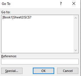
If you double-click on that line it’ll bring up the Go To dialog box which will show you which cell it’s referencing on another sheet:

From here you can click on the item in the Go To box and click OK and it’ll take you to that cell.

If you’re able to see blue arrows or the link to another spreadsheet, then it’s easy to trace where the circular references are . But if you’ve got a large spreadsheet, it may not be so easy spotting where the circular references are, which is why you may need to look at other methods.

One way is by looking at the bottom left corner of Excel, where you’ll see it mention circular references if there is an error:

And if you’re on the same sheet that the circular reference is on, you’ll also see which cell is causing it:

But it won’t be able to show you all of the circular references if there are more than one here as there’s obviously limited space to do that.

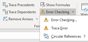
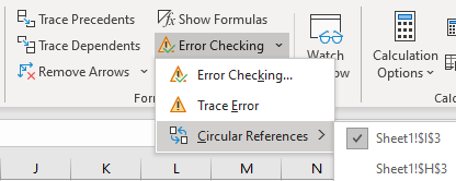
Another way that you can look for circular references is by going to the Formulas tab and then clicking on the down arrow next to the Error Checking button:

Then, click on the Circular References button and you’ll see a list of all the circular references in the workbook:

You’ll notice this way it will also show you which sheets have circular references.

Fixing circular references

Once you’ve identified which cells need to be fixed, then what’s left to do is adjust the cells. If you’ve just made an error then all this may involve is just deleting the contents of the cell entirely or just removing the reference to the cell in order to remove the circular reference.

But in many cases, it’ll involve a formula. And this is where it can get a little tricky as you may need to restructure your formula to ensure it’s not circling back in some way to the original cell. One possible solution can be to add another field as an intermediary to ensure you aren’t trying to do too much in just one formula.


If you liked this post on how to find circular references in Excel, please give this site a like on Facebook and also be sure to check out some of the many templates that we have available for download. You can also follow us on Twitter and YouTube.
hiding values in excel

How to Hide Zero Values in Excel

If you’ve got a big spreadsheet with lots of numbers to look at, it can sometimes be a bit difficult to look at a large chunk of data. That’s where knowing how to hide zero values in Excel can be helpful in reading and analyzing data in Excel. By not seeing the zero values, you can easily focus your eyes on the more important numbers that may need more analysis.

However, it doesn’t have to be just zero values that you hide. Any number that’s insignificant for your analysis can also be hidden. For instance, you can be analyzing a company’s financial performance and choose to hide any movements that are less than 5%. The same principles apply as you would use to hiding zero values. Below, I’ll show you how you can hide not just zero values but any values that you don’t want showing up in your data while still factoring them into totals and any other calculations. You won’t be deleting anything, just masking the information.

First, let’s take a look at how to hide a potentially even bigger nuisance: errors.

How to hide errors on a spreadsheet

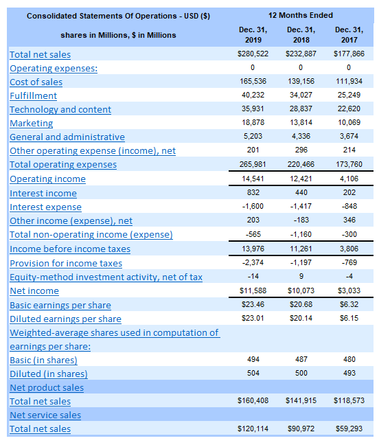
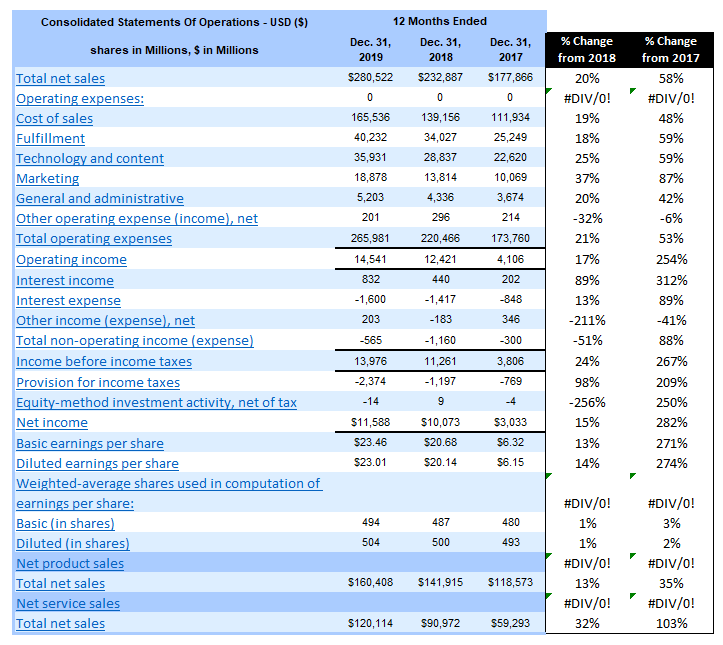
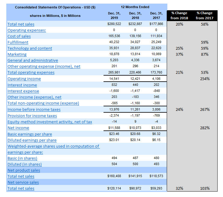
To help illustrate how to hide zeo values in Excel as well as other numbers, I’m going to use some real-world data — Amazon’s most recent annual earnings report, which the company released last month. Here’s the company’s income statement from the past three years:

Amazon's income statement over the past three years in Excel format.

If you’d like to follow along, you can download the data from the SEC. First up, I’ll add a few columns showing the change from 2018 to 2019 and from 2017 to 2019. Here’s how it looks just copying the formulas straight down:

Analyzing Amazon's income statement using Excel with error values showing.

I have divide by zero errors as there are rows that have no data. I could just remove these cells but as with anything in Excel, it’s good to be consistent. Rather than deleting those error values, I can get rid of the errors in one of two ways.

The first is by using an IF statement to say that if the denominator is 0 or blank, to ignore the calculation. The second is just to use an IFERROR statement.

Here’s what my formula looks like for the 2018 to 2019 change:

=C5/D5-1

Where C5 is the 2019 data and D5 the 2018 numbers. I don’t need any parenthesis as order of operations ensures the formula will calculate properly. However, it doesn’t prevent me from getting a divide by zero error. Since the numerator can be blank or zero, what I’ll want to focus on is fixing the denominator in D5. To do this, I can add an IF function that looks at whether the denominator is a number. Here’s what my formula will need to look like to remove that error:

=IF(OR(D5=0,D5=””),””,C5/D5-1)

The formula now checks to see whether D5 is either a zero or blank, and if it is, it returns a blank value. Otherwise, it calculates as normal. Now I can copy this formula down and get rid of the error values.

An alternative way to fix this is by using IFERROR. Introduced in Excel 2007, the function can be an easy way to replace errors on your spreadsheet with another value. In this example, I’m going to use empty quotes (“”). The benefit is obvious: it’s a lot easier to use IFERROR than an IF statement, especially combined with an OR function as well. Here’s what my formula would look like with IFERROR:

=IFERROR(C5/D5-1,””)

It’s a whole lot easier and quicker. I don’t have to worry about the logic and all the reasons why the formula might error out. However, it’s not a perfect solution and here’s why: it will correct errors, but it’s possible they’ll be errors you’re not expecting. For instance, if I copied the data wrong or keyed something over and put text in a field where it should be a number, the IFERROR will correct that and you won’t be able to tell whether it’s blank because it is a divide by error problem or something else. That’s where it can be a little dangerous in using this one-size-fits-all approach to fixing error values. As long as you’re okay with that, it’s a perfectly good approach to fixing the divide by zero errors.

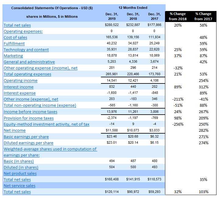
Here’s the data now that it’s been cleared of errors:

Analyzing Amazon's income statement using Excel after error values have been hidden.

That looks a lot better but the problem is that it’s still a lot of percentages to look at and it’s difficult at a glance to see what are the big changes are from the prior year. This is where it’s also important to hide zero values in Excel, as well as low values that aren’t useful for analysis.

How to hide zero values in Excel and other numbers that you don’t want or need to see

In order to hide data, it’s useful to use conditional formatting. If you’re not familiar with how to use conditional formatting, check out this post. Conditional formatting won’t remove or erase any data, which makes it a good solution that will keep all the data and calculations intact.

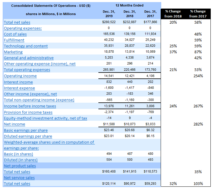
In the Amazon example, there are some pretty large-moving items in the list. Removing zero values won’t do anything and the threshold needs to be big for it to be helpful in hiding the lower values. Let’s start by removing the percentages that are less than 20%. Here’s the formula that I will use in the conditional formatting to accomplish this:

=AND(F5<0.2,F5>-0.2)

Column F is where the % Change from 2018 values are. I need to use the AND function because if I just look at anything that’s less than 20% this will also capture negative movements that are more than 20%. And for now, I want to keep those. I want to remove anything that’s between -20% and +20%, which is what the above formula will capture. If I was only looking to remove the zero values then the formula would be as simple as F5=0.

The next step is to adjust the formatting so that the cell font is white. Changing the color is an easy way to hide a cell’s value if it’s on a white background. While that data is still there, it won’t be visible:

Analyzing Amazon's income statement using Excel with error values fixed and low values hidden.

It creates a lot more white space, allowing me to see a lot more of the bigger values. The problem that I notice, however, is that there are some low values that are creating big movements in percentage. I can go a step further and create another conditional formatting rule that will also ignore the percent change for any item in 2019 that was less than $1 billion (1,000). This is how that formula will look:

=$C5<1000

I need to freeze column C because the conditional formatting will be used for the other change column as well and I don’t want the reference to move. Now, with this adjustment, it makes a much bigger difference and helps me narrow in on fewer items:

Analyzing Amazon's income statement using Excel with error values fixed and low values hidden.

I can see that the significant changes from 2018, besides the totals, were in sales, technology and content, and marketing. However, since the growth rate from 2017 is even higher, I’ll need to adjust those percentages to also ignore anything that’s not at least a 50% improvement. Here’s how that formula will look (note that I’ll only apply it for the % Change from 2017 column):

=AND(G5>-0.5,G5<0.5)

Remember, since I’m analyzing percentages, these figures need to be in decimal point. Otherwise, I would be using whole numbers. With those changes, this is how my data looks:

Analyzing Amazon's income statement using Excel with error values fixed and low values hidden.

Now I’ve also got a reasonable amount of items I can focus on for the % Change from 2017 column. In addition to the same items increasing from 2018, I notice that fulfillment costs have also shown a significant increase over two years.

The conditional formatting works great in clearing out numbers that I don’t want to see. However, there’s just one small problem…

Analyzing Amazon's income statement using Excel with hidden values showing on a dark background.

If I change the color to anything that isn’t white, those numbers that I hid become visible again. That leads me to another all-important section:

How to hide values in Excel that are on different background colors

You can create conditional formatting rules to address other background colors but that’s just not practical. If you use lots of colors on your spreadsheet the last thing you want to do is create a rule for every different color and make sure the cells are hidden in the same font color. There’s also a problem if someone changes the color too.

That’s why using font color to hide values in Excel isn’t a good idea. The good news is that there’s a much easier way to hide values that doesn’t involve you having to try and match up the color.

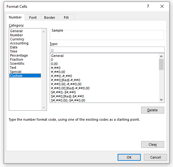
Rather than changing the color, what you should do is use a custom number format. Simply use three semi-colons and that will do the trick:

Choosing a customer number format to hide zero values in Excel.

Without going into the details of the different formats you can use, by using three semi-colons you’re telling Excel that you want no formatting to be used whether the amount is positive or negative. Now, my hidden data remains hidden regardless of the background color:

Analyzing Amazon's income statement using Excel with hidden values no longer showing on a dark background.

Now you don’t have to worry about background colors and can easily hide your data in any context.


If you liked this post on how to hide zero values in Excel as well as other values, please give this site a like on Facebook and also be sure to check out some of the many templates that we have available for download. You can also follow us on Twitter and YouTube.
error1

Formatting and Removing Errors and Zero Values

Often times in a data set you’ll have to handle with errors that can wreck your data, especially if you need to do any analysis on it. There are several ways that you can handle errors so that they don’t show up in your data.

IFERROR

The first method is by using the IFERROR function, which allows you to easily replace the error with whatever you want in its place. If you want a numerical value, you may want to put in a 0, otherwise you can just leave it blank. 
I’ve purposely added various types of errors to my data set:
Here is one of the formulas that’s causing an error:
=VLOOKUP(D7,L:L,1,FALSE)
In the above example, I could use the formula =IFERROR(VLOOKUP(D7,L:L,1,FALSE),””) to replace the error with a blank. I could also put a 0 in its place instead of the “”. 
ISERROR

In older versions of Excel (2003 and earlier), the IFERROR function is not available. However, what you can use is a combination of the IF and ISERROR functions. To recreate the same formula as above, we can use the following:
=IF(ISERROR(VLOOKUP(D7,L:L,1,FALSE)),””,VLOOKUP(D7,L:L,1,FALSE)
The disadvantage of this method is you have to repeat your original argument. First, you are checking if the value is an error, if it isn’t, then you have to repeat the formula again to save the value. It’s not terribly efficient, and likely why we saw the IFERROR function introduced in newer versions of Excel.
Using the IFERROR or IF(ISERROR()) functions can be useful for eliminating errors, but sometimes it may not be helpful for dealing with specific ones. For example, if your cell is blank or it has an error and is made to look blank, you won’t be able to tell the difference just by looking at it. The danger is that you may assume it’s a different type of error.
ISNA

What you can also use is the ISNA() function, which can tell you if the cell returns the #N/A error. This way you can trap this error specifically, rather than everything that can be captured by the ISERROR() function.
Getting Rid of Zeros

If you’ve used a lot of error-handling functions and replace your errors with zeros, you could up with a lot of zero values on your spreadsheet:
The problem if you have a lot of zeros on your spreadsheet, is it can sometimes be a distraction away from what you really want to see – the non-zero values. There are two ways you can get rid of the eyesore:
1. Change the format to Accounting. Doing this will remove the zero values and replace them with a dash, which makes it a bit easier to skip over when doing a review:
However, you may not want to use the Accounting format, and that leads me to the other option:
2. Conditional Formatting. Refer to this post on how to setup rules for this. What I normally do in these cases is set the zero value cells to a light gray color font so that they do not attract your attention:
Common Types of Errors

Here’a list of some of the common types of errors you’ll find in Excel:
#REF: This is an error that you’ll incur if your range doesn’t go far enough and the error relates to your reference. For example, consider a VLOOKUP formula that extracts from column number five but you only specified a range that had four columns, that would result in a REF# error.
#N/A: You’ll get this error if your VLOOKUP or MATCH formula is correct, but the value you’re looking up isn’t found, and hence, not available. However, there’s other contexts it can apply to, and it just means that it wasn’t able to find the value you were looking for. 
#VALUE: This error normally shows up when there is an issue with your actual calculation. For instance, if you’re trying to multiply a number by a field that has text. 
These are just a few examples of the errors that you’ll encounter, but these are also likely the most common that you’ll come across.
Inventory count sheet showing data by product number.

How to Sort Data in Excel Without Messing Up Formulas

If you have a formula that involves multiple sheets and you later sort that data you may notice your cell references are now out of order and need to be corrected. It can be frustrating and dangerous because you may not realize your formulas are now calculating different cells.

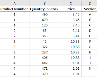
For example, I have created a sheet called InventoryCount and another called Total. The InventoryCount sheet acts as a tally of all the locations a certain product number is found:

Inventory count sheet showing data by product number.

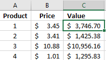
On the totals sheet, I have a summary of these product numbers using a SUMIF formula that multiplies by the price.

A summary of the inventory values.

The formula in the highlighted cell above is as follows:

=SUMIF(InventoryCount!A:A,Total!A2,InventoryCount!B:B)*B2

The formula in the price column for product 1 is:

=VLOOKUP(A2,InventoryCount!A:C,3,FALSE)

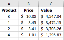
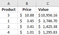
Both formulas are referencing the InventoryCount sheet. The formulas in the value column are correct. But let’s say that I want to sort that column by values. If I sort in descending order, this is what I get:

Inventory data after applying a sort.

The values are not only not correctly sorted  (product 1 is lower than product 2’s value) but the values have changed. If you look at the values before the sort product 3 dropped from 10,956.16 to 4,547.84. There is nothing glaringly obvious that the calculation is now completely incorrect so you can imagine the danger when dealing with lots of data that such a sort could make your data get altered. The formula for the value in product 1 now looks like this:

=SUMIF(InventoryCount!A:A,Total!A2,InventoryCount!B:B)*B3

It is still referencing A2. So technically the formula is still correct, the problem instead is product 1 is no longer on row 2, it is on row 3. The assumption that the value in row 3 relates to the product on row 3 will now be incorrect.

So why did this happen? Notice that the price has not changed for any of these products, Product 1 was $3.45 before the sort, as well as after. This column still is correct in relation to its corresponding products.

If you go back and look at the two formulas (price and value) you will notice on key difference: the cell referenced on the current sheet (Total) for the price does not mention the sheet name, however on the value formula it does.

This is the original formula to calculate the value:

=SUMIF(InventoryCount!A:A,Total!A2,InventoryCount!B:B)*B2

The Total! reference is causing the sorting issue and needs to be removed. The updated formula becomes:

=SUMIF(InventoryCount!A:A,A2,InventoryCount!B:B)*B2

Now if I apply the same logic to the other formulas in the value calculation and sort the data in descending order, below is the result I get:

Inventory data after applying a sort.

The values are back to what they were at the start and product 3 is the highest as it was initially. Except now they are correctly sorted in descending order with the product number correctly being referenced in column A.

So the lesson here is that if you are using formulas with multiple sheets get rid of the sheet reference when referencing a cell on the same sheet as the formula is on (Excel inserts this reference automatically as you switch from one sheet to the next). Otherwise, if you or anyone else sorts the data the calculations will not be on the correct rows.


If you liked this post on How to Sort Data in Excel Without Messing Up Formulas, please give this site a like on Facebook and also be sure to check out some of the many templates that we have available for download. You can also follow us on Twitter and YouTube.