Excel is a powerful tool, but even the most experienced users encounter errors like #N/A from time to time. This error can be frustrating, but it’s actually Excel’s way of saying it can’t find the information it’s looking for. Let’s break down why this error happens, and how to fix it.
What does #N/A mean?
The #N/A error occurs when a formula cannot find a value it’s supposed to look up. This commonly happens with lookup functions like VLOOKUP, HLOOKUP, INDEX and MATCH, or XLOOKUP.
Common Reasons for #N/A Errors
When a value isn’t found in your lookup formula, there are multiple possible reasons why that might happen. Here are some of the most common issues:
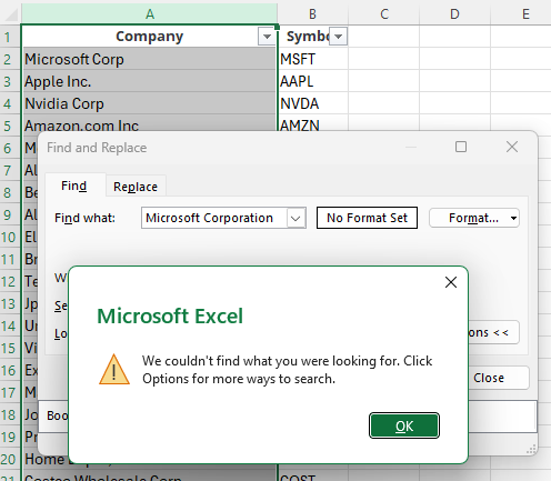
The value isn’t in the lookup range. The simplest reason is that the value simply isn’t there. Perhaps the value you’re looking for is spelled differently than what you’re searching for, or it just isn’t contained within the data set. An easy way to check for this is to use the CTRL+F shortcut and manually search for the value. If it isn’t found, you’ll get a message saying the value isn’t found. If it is, then it’s likely one of the other reasons that’s causing the error.

In the above error, ‘Microsoft Corporation’ isn’t found because the text in the range is just ‘Microsoft Corp’
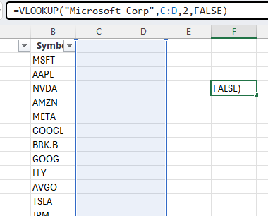
The range or table being searched is incorrect. In this situation, your value exists but it can be that you’re looking in the wrong place. For example, if your data set is in columns A:B but you’re looking at values in C:D, then the value won’t be found. The only way to catch this is to manually look at your formula. By clicking into the formula, it will highlight the range it’s looking at. If it doesn’t look like you’ve selected the right area, that can explain why you are encountering an error.

The data types are not the same. In this situation, you may be searching for a numerical value of 1 but the actual value is a text value of 1. This can be a more challenging issue to uncover. However, by using the CTRL+F function you can confirm if the value is indeed found. And if it is found, what you can do is use a formula to check if the values are an exact match. Suppose your lookup value is in cell A1 and the matching value is in cell D100. You can enter the following formula below, to confirm whether it is an exact match:
=A1=D100
If there is an error, that means the data is not the same. At this stage, you may want to do a closer analysis of the values to see if there are any extra characters. You may also want to use the ISNUMBER function to check whether one value is reading as a number and the other as text, as that could be resulting in the #N/A error as well.

If the result of the ISNUMBER formula is FALSE, that tells us that the value is not a number despite it appearing to be.
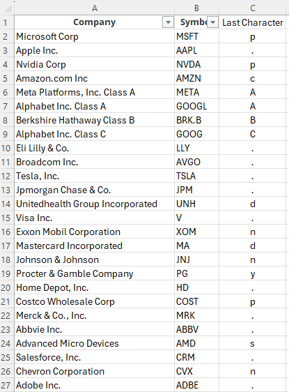
There are trailing spaces. If your data type is the same and it looks like everything should be matching, then it may be an issue that you have a trailing space, either in your lookup value or the value which it should be matching to. An easy way to check for trailing spaces is by using the RIGHT function. If you don’t specify the number of characters you want to extract from the right, it will by default grab the last one. Then, if you see the formula returning characters, you know there are no trailing spaces. If, however, there is a blank value, this would be confirmation that a blank space exists at the end, and it could be interfering with your lookup.

In the above example, column C shows the last character. While there are letters and punctuation, there are no blank values shown.
How to use formulas to suppress #N/A errors
If all else fails and you can’t find the reason for the #N/A error, or it’s not possible to eliminate it without drastically changing your spreadsheet, or you simply don’t have the time to look through all the possible reasons, then you can use formulas to suppress the errors for the sake of eliminating them. There are two options here.
IFNA
The IFNA function can replace the error value with a different value of your choosing. You may want to simply have an empty value, perhaps a 0, or just a different message altogether. In the following formula, I’m using the IFNA function to return a text value of “Not Found” if the value in F4 is not found within column A:
=IFNA(VLOOKUP(F4,A:B,2,FALSE),”Not Found”)
If you encounter any other error, then you’ll still see an error. This function will only suppress #N/A errors.
IFERROR
The IFERROR function works similarly to the IFNA function but the key difference is it will suppress any and all errors. You can deploy it in the same way as you would the formula above:
=IFERROR(VLOOKUP(F4,A:B,2,FALSE),”Not Found”)
The advantage of using this function is it will remove any errors. But that can also be a drawback because if there are different issue causing the error, it won’t be evident, and that can mask other problems within the spreadsheet.
If you like this post on How to Fix #N/A Errors in Excel, please give this site a like on Facebook and also be sure to check out some of the many templates that we have available for download. You can also follow me on Twitter and YouTube. Also, please consider buying me a coffee if you find my website helpful and would like to support it.

