

In a previous post, I covered how to add checkboxes. Now, I’m going to go a step further and show you how you can create a form in Excel from start to finish. And at the bottom of the page, you can download a file that you can use for your own custom forms. It will incorporate, list boxes, checkboxes, validation rules, and allow you to move the data onto a separate sheet. For now, let’s start from scratch.
Step 1: Determine the data you want and how it should be entered
The first step in creating a form in Excel is determining what information you want to collect. In this example, I’m just going to include name, address, city, state, email, a checkbox to confirm if it is okay to contact the person, a rating, and an area for comments. It is also important to determine how users should enter these values. While it’s easy to leave everything as text, that can make it difficult to ensure someone doesn’t enter invalid data. And if the data is not useful, it will defeat the purpose of the form.
Here are the types of inputs I’m going to use for my fields:
- Name: Text
- Address: Text
- City: Text
- State: List box
- Email: Text
- Contact confirmation: Checkbox
- Rating: Radio button
- Comments: Text
Next, let’s work on the form’s design.
Step 2: Designing the form and creating the inputs
One thing I did to help make the form cleaner from the beginning was to turn off gridlines. You can do that by going to the View tab and unchecking Gridlines under the Show group:
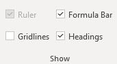
This will make your form look more like a form and less like a regular Excel sheet. Another thing you can do is in that same section, unselect the Formula Bar and Headings, which will add more white space and are unnecessary if someone is just filling in a form. However, you may want to save this for the end when your form is done.
Since an Excel form can come in all shapes and sizes, the one thing that may help you in the design process is to set every column to a width of 2. This way, it will be easier to maneuver in case one field needs to be bigger than another without having to try and force everything to be a similar length.
As for the input fields, there are a few things you will want to do:
- Make sure they are long enough. A good way to test this is by entering a long value, or what you might think will be the longest value into each field and then adjusting its length so that everything displays correctly.
- Assign a named range. This is useful to keep things organized and it will make it easier for you to refer back to the field later on if you only have to remember its name, as opposed to its cell reference.
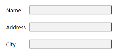
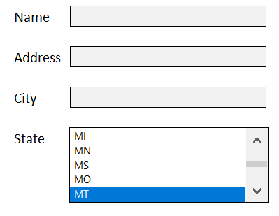
Now, let’s move on to creating the fields in the Excel form. What you can do for text entries is to just add some outlining and highlighting to existing cells. A subtle light grey can be a good way to indicate that is an input value. And I’ll also add a border to help make these fields stand out. If you set the column width to 2, you’ll also need to merge the cells as needed.
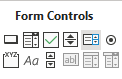
For the State field, I’ll go back to the Developer tab where I will select the option for a List Box from the Form Control section — which is next to the Radio Button on the right. When in doubt, you can hover over each control to see what it is.
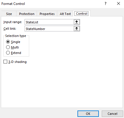
After creating the List Box, I need to populate the list plus link to a cell where the selected value should go. I’ll start with creating a range of cells for all 50 states and then assign a named range for them called StateList.
Then, I will set up a named range called StateNumber for the linked cell. Here is what the List Box control shows when I go into Format Controls and select the Controls tab:
But this is not enough as the list box returns a number, not the state’s initials. I will need another cell to pull that in. I created a named range for State and here is what my sheet looks like:
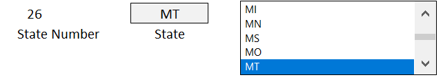
In the list box, I selected MT, which returns a value of 26 in the StateNumber range. To extract the state’s initials, I need to use a formula to get that. Since I’m getting the data from one column, I’m just going to use the INDEX function. Here is what the formula in the State named range looks like:
=INDEX(StateList,StateNumber,1)
It is looking at the StateList and pulling out the row that relates to the StateNumber. Since MT is the 26th selection, that is the value that gets returned. So now my List Box is working correctly. What I like to do with these named ranges is to hide them so that the user doesn’t see all these intermediate steps. All it takes is to just move the List Box over top of these cells:
And just like that, the user only sees their selection and not the calculations afterwards. You could certainly use a drop-down list for states but I thought I would try something different and more user-friendly for this example.
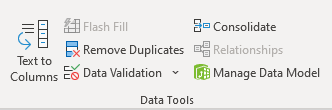
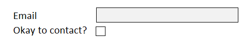
Next, let’s go to the email field. This can be tricky because although you want this to be text, you also want to control what a user enters to avoid a possible error. You can’t guarantee the email will be correct but you can take steps to at least prevent some errors. The key here is going to be to create a data validation rule. There are two things that should be present in email addresses: the @ sign and a period. To create a data validation rule, select on the cell and click on Data Validation under the Data tab:
There are many rules you can set up such as limiting the entry to fall within certain dates, making sure it is a whole number, or that it is from a drop-down list. But this situation is unique and will require a custom formula.
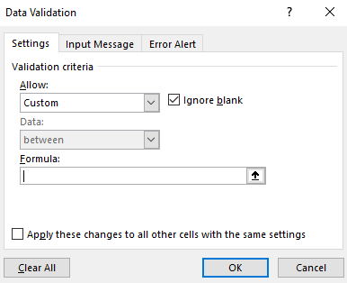
To check for both the period and the @ sign, I will need to use the FIND function and check that the value is a number (which means that it was found). Here’s how that looks inside of an AND function:
=AND(ISNUMBER(FIND(“.”,Email)),ISNUMBER(FIND(“@”,Email)))
Since I set the field to a named range of ‘Email’ it is easy to reference it without worrying about whether I have selected the right cell. If I put this calculation in the formula section, now you won’t be able to enter a value that doesn’t include both a period and an @ sign. In addition, you can also specify the error alert and determine what pops up if someone enters something different that violates these rules. However, that’s not necessary as they will get an error anyway.
Now, I’ll add the checkbox for the email. This again comes from Excel’s Developer tab and the Form Control section. Simply select the checkbox and set up a linked cell. If you want more details on this, refer to the link at the top of this post for a more detailed outline of how to add checkboxes. I have positioned the checkbox right below the email field:
Next, I’ll add some radio buttons to allow someone to leave a rating. These are useful if you want to specify a number. Here I will go back to the Developer tab and create some radio buttons and re-size them so they don’t take up much space. Unlike the other controls, you will want them to all have the same linked cell; the purpose of radio buttons is that there is only one selection. Here is how I added them, just below the numbers that they refer to:

The radio buttons will automatically increment on their own so if you don’t pay attention to what order you’ve added them in you may get some unexpected results.
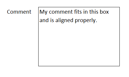
Lastly, I will add a large comment box where people can leave detailed comments. This can just be a large merged cell that takes up more space.
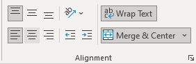
But the one thing you will want to do is make sure that Wrap Text is selected so that the comment fits in the box. And you will probably want to align it so that it is in the top left corner of the cell:
Then, when I enter the text it looks correct:
Here is what my completed form looks like:
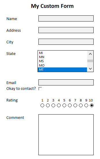
It looks good, but we are still not done. Something needs to happen with these inputs otherwise the information goes nowhere. Let’s go over that next.
Step 3: Storing the data from the form in an Excel sheet
If you are sending just a single form over for someone to enter data in, what you can do is create an output page that will link to these values. Since they are all named ranges, you can easily reference back to them as such:
=Name
In the above example, if you created a named range called Name for the first field, it will pull in the data from there. On an output sheet, you might have formulas and values that look like this:
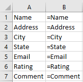
In column B I am showing the formulas. You can keep this tab hidden if you want it out of sight. You can even go one step further and make them very hidden.
Not sure whether your fields should go horizontally or vertically? In most cases, you’ll actually want them going across the top. When in doubt, consider the number of fields you have versus how much data you will be entering into the sheet. If you will have dozens of results that you will need to populate (or more), you probably don’t want to be cycling through that many columns; rows are easier to scroll through and that’s why it will probably make more sense for the fields to go across the top.
Once you have your output tab set up, you can copy the values you get back from these forms and start populating a database.
But what if you are doing data entry and need to make these entries multiple times and need the data to push to the output tab automatically after each entry? This is where you will need to set up a macro and need a button to trigger this movement onto the output tab. If you’d like to see how that code might work or just want a ready-to-use file that you don’t have to mess around with, you can download this free template.
The template will grab the input values and based on the named ranges, it will populate them in the output tab once you click the Post button on the main page. If there isn’t a named range that matches to a header on row 1 on the output tab, the data just won’t get copied over. Give it a try!
One additional step you may want to consider is locking down the form in Excel to make sure people don’t accidentally move things around or delete any formulas. You can protect the workbook and the individual sheets do that. Click here for information on how to lock cells.
If you liked this post on how to create a form in Excel, please give this site a like on Facebook and also be sure to check out some of the many templates that we have available for download. You can also follow us on Twitter and YouTube.
