Google Sheets provides investors with a great way to pull in stock prices, ratios, and all sorts of information related to stocks. Pulling in a stock’s history, for example, can make it easy for you to calculate a stock’s relative strength index, or create a MACD chart. But doing any sort of analysis for multiple stocks at a time isn’t easy. One way around this is to create a macro using Google App script that can automate the process for you and cycle through multiple stocks. Don’t know how to do it? No problem, because below I’ll provide you with a setup and a code that you can use.
First, I’ll go through creating the file from scratch and how it works.
Setting up the template
In this example, I’m going to find the stock’s largest value for a specific period. To start, I’m going to use the GOOGLEFINANCE function to get the stock history going back to Jan. 1, 2020. In the below example, I’ve got the price history for Meta Platforms, aka Facebook:
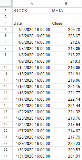
In cell B1 I’ve put a variable for the ticker symbol. This is to avoid hardcoding anything in the formula. This is important to make the process easy to update. In the macro, I’m going to cycle through ticker symbols. In Cell E2, I also have a formula that grabs the largest value in column B (the closing price):
=MAX(B:B)
However, this is where you can put your own formula or the results of your own calculation. Whether it’s a minimum, a maximum, or some other computation you want to do, you can put the results of that calculation here. This is the cell that will get copied during the macro.
Then, in column G, I have a list of the stocks that I want the macro to cycle through:
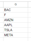
As long as it’s a valid ticker symbol that the GOOGLEFINANCE function recognizes, you can enter it in this column. You can expand it as far as you like. However, if the macro goes on for too long then it will eventually time out and stop. If you want to cycle through every stock in the S&P 500, it is possible, but just be aware that you’ll likely have to do it in chunks. When testing it myself, I estimated I could do somewhere in the neighborhood of 200+ stocks in a single run. Once done, I copied the values onto another place on the spreadsheet with the values, and then replaced the stocks in column G with the next batch.
In Cell J1, I also have a variable called tickercount. This is a helper calculation to make the macro efficient. Instead of it having to count the number of stocks in my list, I provide it for the macro — anything to make it run quicker.
The Apps Script Code
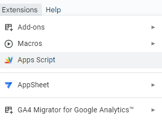
Now it’s time for the code to make this all work. To add code to your Google Sheet, select the Extensions menu and select Apps Script
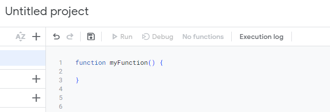
Once in Apps Script, you can setup a new function. You should see the following:
Here’s the entire code that you can use based on my setup:
function myFunction() {

var sht = SpreadsheetApp.getActiveSheet();
var lastrow = sht.getRange("tickercount").getValue();

for (i=1; i<=lastrow;i++) {

  //change ticker
  sht.getRange('B1').setValue(sht.getRange('G' + i).getValue());

  //copy maximum value
  var result = sht.getRange('result').getValue();

  sht.getRange('H' + i).setValue(result);


}
}
Here’s a brief explanation of how the code works:
- It begins by selecting the active sheet.
- It determines the last value based on the ‘tickercount’ named range.
- It loops through the values in column G.
- It takes the value in column G and pastes it into cell B1 (the ticker variable).
- The macro then gets the value from cell E1 (it has a named range called ‘result’)
- It pastes the value of the result into column H, to the same row that the stock ticker was on.
If you leave my setup the way it is, what you can do is do any of your desired calculations on another part of the worksheet. As long as it doesn’t interfere with the ticker list or any of the ranges used in the macro, then you’re fine. You can also adjust where the cells are if that makes it easier. For example, you could move the ‘result’ named range from E1 to somewhere else in the spreadsheet. With a named range, you don’t need to worry about updating the cell reference.
Running the macro
A final part of this macro is actually running it. You need a way to trigger it. In my example, I’m using a button. This makes it easy to see what you need to click on for the macro to run. Here’s how you can create a button in Google Sheets and assign a macro to it:
1. Go to Insert and select Drawing
2. Create a shape, add text to it, and whatever colors/formatting you want. Then click Save and Close.
3. Select the button and click on the three dots on the right-hand side, where you will see an option to Assign Script.
4. In the following dialog box, enter the name of your function (don’t include the parentheses). The default function in Apps Script is called myFunction() and if that’s the macro you want to use, then you would just enter myFunction and click on OK.
If everything works, now when you click on your button, the macro will run. Check for any error messages to see if you run into any issues. If you need to edit the button afterwards, right-click on it first so that you don’t accidentally trigger the macro.
One thing to note is that when you run a macro on a Google Sheets file for the first time, you’ll be given a warning about doing so:
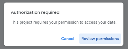
Click on Review permissions and select your Google account. You’ll get the next warning, saying that Google hasn’t verified this app and you’ll need to click on Advanced to continue despite the warnings. This is similar to the warnings you encounter in Microsoft Excel when enabling macros. Once you proceed and click on Allow, the macro will proceed to run.
Here’s how it looks in action:
Download my loop macro template
If you’ve gone through this post and run into issues or it is too complicated for you, feel free to download my loop macro template. Since it’ll create a copy for your use, you can modify it however you like to suit your needs.
If you like this post on Loop Through Stocks in Google Sheets With a Macro, please give this site a like on Facebook and also be sure to check out some of the many templates that we have available for download. You can also follow me on Twitter and YouTube. Also, please consider buying me a coffee if you find my website helpful and would like to support it.

