Excel’s new functions help make it even easier to analyze and extract data efficiently and effectively. One example is extracting a list of unique values from a list. What you can also do is sort that list. Plus, you can then put all those values into a single cell, with each value separated by a comma. Data in the form of a comma-separated value (CSV) can make it easy to compile data into one place, without taking on too much space. In this article, I’ll show you how we can combine all this Excel functionality into one supercharged Excel formula that can do everything I’ve mentioned thus far. Let’s get started.
How to create a list of unique values for a specific criteria
For starters, let’s get a list of unique values that meet a certain criteria. While pulling unique values isn’t terribly difficult in excel and there many ways to pull unique values, I’m going to show you how we can extract unique values that meet a given criteria. Here’s the data set I’ll be working with for this example:

It’s a straightforward list that includes a client number (column A) along with invoices (column B). But if I want to include just a list of the unique values relating to client 1000, the UNIQUE function on its own won’t help me with that. I need to apply a criteria first. To do this, I’ll first use the FILTER function. Using that function, here’s how I can grab all the values relating to client 1000:
=FILTER(B:B,A:A=1000)
The first argument in the formula is where I want to extract values from. The second argument pertains to my criteria, which is based on the values in column A. With this formula, this is my result:

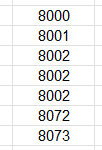
I get a list of values. But the problem is I have repeating values — invoice #8002 shows up multiple times. But I can put that formula to generate that list within the UNIQUE function:
=UNIQUE(FILTER(B:B,A:A=1000))
Now I have a condensed list which only includes unique values:

If your data isn’t sorted, you can also put this within the SORT function:
=SORT(UNIQUE(FILTER(B:B,A:A=1000)))
Now you have a formula that filters out data, grabs the unique values, and sorts them. It’s a busy formula. But it’s about to do even more.
Putting the list into a CSV format
As of now, the data is in a list. That’s not a convenient format because the danger is that you may have clients which have only a few invoices, perhaps none at all. Others, meanwhile, might have a dozen invoices. If you are creating arrays, they will inevitably vary in size, and the you’re left with a spreadsheet that doesn’t have much consistency to it.
To get around that, you can put your data in a CSV format. By doing so, you can ensure all of your data is contained within just a single cell.
Here’s the step-by-step process as to how you can put your data into a CSV format:
1. Use the TEXTJOIN function and use a “,” as you first argument. The first argument of this function tells you how you want to separate your data. By indicating a comma, you’re already setting up the result to be in a CSV format.
2. Set the next argument to TRUE. The second argument is whether you want to ignore empty values. You’ll likely want to ignore them, otherwise, you will have blank spaces between your commas.
3. Include your list of values. This is the data that you want to convert into a CSV.
Here is what the complete formula looks like, with step 3 relating to the formula we created at the end of the previous section:
=TEXTJOIN(“,”,TRUE,SORT(UNIQUE(FILTER(B:B,A:A=1000))))
Now the result is the following:

The list of unique invoice numbers is now within just a single cell. And each invoice is separated by a comma.
But let’s make this formula more dynamic. It should be able to generate a list based on each client, in the following table:

With the client values in column D, starting with cell D3, this is how I can adjust the formula so that it is not referencing a hardcoded invoice number:
=TEXTJOIN(“,”,TRUE,SORT(UNIQUE(FILTER($B$3:$B$101,$A$3:$A$101=D3))))
Using that formula, the table will now populate the list of unique invoices for each client:

If you like this post on How to Extract and List Unique Values in Excel Into CSV Format, please give this site a like on Facebook and also be sure to check out some of the many templates that we have available for download. You can also follow me on Twitter and YouTube. Also, please consider buying me a coffee if you find my website helpful and would like to support it.

