How to Create an Inflation Calculator in Excel

Want to know how much something was worth decades ago? Or how much something costs in today’s dollars? Using inflation data, you can estimate that. And in this post, I’ll show you how you can create your own inflation calculator template in Excel. I’ll also provide you with my free template.

Getting the data

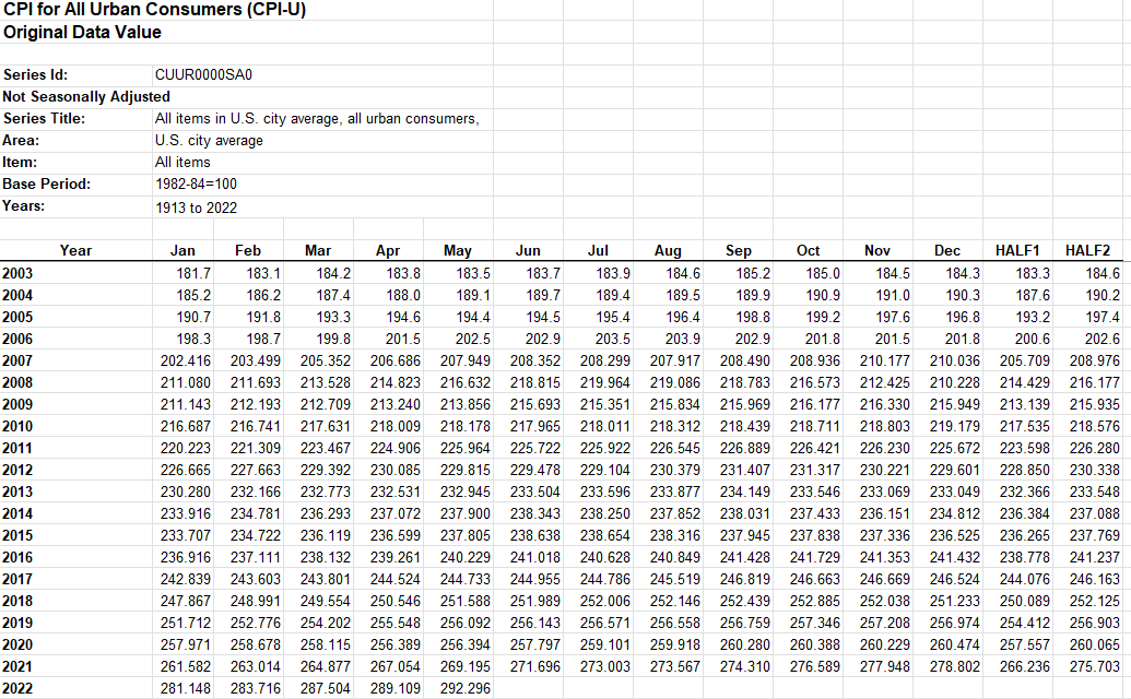
You can get inflation data going back to 1913 from the U.S. bureau of Labor Statistics. There’s an xlsx file there that I’m going use that will be the source for my calculations.

Once in Excel, you’ll see the data is neatly formatted by both year and month:

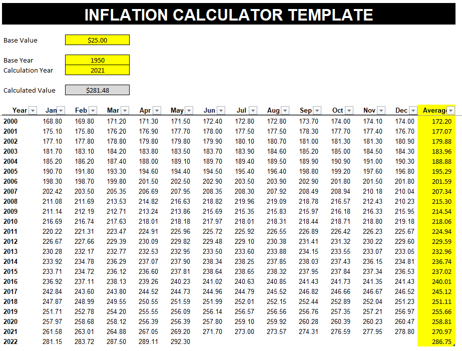
This data will get updated so over time you may want to get the latest figures so that your calculations are as accurate as they can be. The data has 1st half and 2nd half numbers but one thing I will do is also add the 12-month average. I’ll add a new column so that it just averages the values. In most cases, you’re probably just going to want to compare data from one year to another.

Next, I’ll convert the data into a table. To do this, click anywhere on the data set and under the Insert tab, click on the Table button. Excel should auto-detect the range but if it doesn’t, you can adjust it. In my template, I’ve named this table tblInflation. It includes the average, which will auto-update as new data is included.

Setting up the calculations

The next step involves creating the inputs, doing the lookups, and then calculating the value. There are three inputs I’ll set up: the base value, base year, and the calculation year. The base year and value will act as the starting points and will convert to a calculated value based on what the calculation year is.

To determine the impact of inflation, I’ll use the base and calculation years to find their respective index values. To do that, I’m going to use a formula that includes INDEX & MATCH. Here’s what it looks like for the base year:

=INDEX(tblInflation[Average],MATCH(BaseYear,tblInflation[Year],0),1)

In the table, I’m extracting the value from the Average column and I will be matching the BaseYear (the named range for my input) against the values in the Year column. I’ll use a similar formula to extract the index value for the calculation year. I’ve put these index values next to my inputs but will hide them later:

In 1913, the index average was 9.9 and for 2022 it was around 286.8 (based on the data that’s available thus far). If I take the index value from the calculation year and divide it by the index value from the base year, that tells me the prices are approximately 29 times what they were back then. That comes out to a percentage change of 2,797%. This leads me to the next part of the equation: determining the new price, or as I’ve referred to it in my template, the ‘Calculated Value.’ The formula for this output is as follows:

=CalculationIndex/BaseIndex*BaseValue

In the case of the above inputs, it’s doing the following calculation:

=9.88/286.75*100

This gives me a value of $2,901.40. That means something that was worth $100 in 1913 would be worth $2,901.40 in 2022. I can also do the reverse calculation. I can work backward and answer the question of how much would something in today’s dollars be worth back then. To do that, I would enter the following inputs:

The calculated value is the $100 that I started with in the previous calculation.

My templates is complete and all that’s left at this point is just to add a header and modify some formatting:

You can download the inflation calculator template here.

If you liked this post on How to Create an Inflation Calculator in Excel, please give this site a like on Facebook and also be sure to check out some of the many templates that we have available for download. You can also follow us on Twitter and YouTube.