H2eDynamicChartRanges

How to Create a Dynamic Chart Range in Excel

Do you have a chart that you want to easily modify the range on, without needing to manually select the data again? Thanks to a new Excel feature, there are now multiple ways you can do that.

1. Creating the chart range as a table

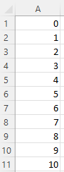
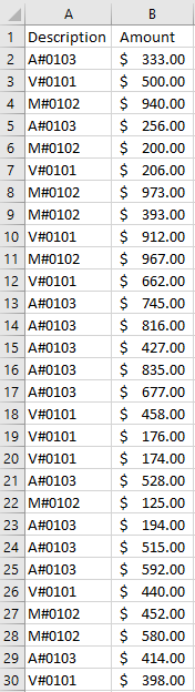
One way you can set up a dynamic chart range in Excel is to put your data into a table. That way, Excel can easily see where you data starts and ends. Suppose you have the following data:

Table showing sales by store.

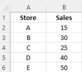
You could show this on a chart but if you needed to add or remove rows from it, your chart wouldn’t automatically re-size. If you deleted data, then there would be gaps on your chart. And if you just added a row, Excel wouldn’t add it to your chart unless you re-selected your range.

To fix this, you can convert you data into a table. To do this, go to the Insert tab on the ribbon and select Table. You may see some default formatting applied afterwards:

Data that has been converted into a table.

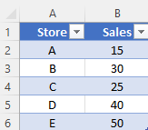
Tables will automatically expand as you add or remove data, and formulas will also copy down by default to any new rows. Currently, this is what my chart looks like for this table:

Chart showing sales by store.

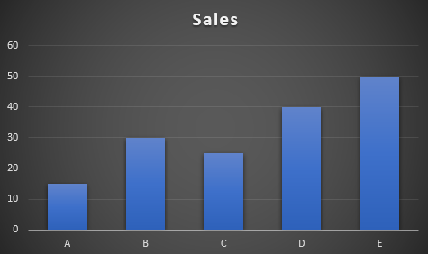
In the below example, you’ll see data being added and removed from the table, and the change to the corresponding chart.

2. Using an array

If you don’t want to convert you data into a table, Excel has now made it possible to dynamically update your chart using just an array, which is new functionality. From the earlier example, I can create an array that populates the data using the following formula:

=OFFSET(A1,0,0,COUNTA(A:A),2)

The first argument reflects the starting point of the data. The next two are left as zero since I don’t want to actually offset the range. The last two arguments indicate the size of the array, and this is key to making the chart automatically update.

By using the COUNTA function, the formula will automatically adjust based on the number of items in that column. That way, if you add or remove items, the offset function will adjust your range. The last argument (2) indicates that the data set is to two columns wide. Now by updating the source data, both my array will update and so too will the chart:

Arrays are not new to Excel but the ability for them to dynamically update a chart is a new feature. As of now, this feature hasn’t fully rolled out to the public and is only available through the Office Insiders program. To get access to that, you can sign up to be an Insider (free of charge) and then moving forward, you will have Excel’s latest and greatest features as soon as they become available.


If you liked this post on How to Create a Dynamic Chart Range in Excel, please give this site a like on Facebook and also be sure to check out some of the many templates that we have available for download. You can also follow us on Twitter and YouTube.

H2Esmallestnonzero

Find the Smallest Non-Zero Value in Excel

Do you need to find the smallest value but want to skip over any zero values? In this post, I’ll show you how you can do just that. The MIN function in Excel does a good job of finding the lowest value but if you have any zero values, those will get included in the result. So how can you get around the issue and get the smallest non-zero value? There are multiple ways you can accomplish this.

Using an array function

An array function allows you to evaluate each cell and that can tell the function whether to include it in its calculation. In the following example, I have a list of the numbers from 0 through to 10:

Numbers 0 through 10 are listed.

By just using the MIN function on that entire range, I will get a value of 0 as the result. However, you can get around this by embedding an IF statement within your MIN function and then turning the formula into an array. The regular MIN function would look as follows:

=MIN(A1:A11)

The IF statement will look to see if a value is not equal to 0 by using the “<>” operators:

=IF(A1:A11<>0,A1:A11)

The IF function evaluates every cell and if it’s not equal to 0, then it returns the value. Here’s how it looks embedded within the IF statement:

=MIN(IF(A1:A11<>0,A1:A11))

The result of this formula is a 1, as it will ignore any 0 values. If you’re running an older version of Excel that doesn’t calculate this correctly, you will need to use CTRL+SHIFT+ENTER to convert this into an array formula and so that you have the curly braces around it as such:

{=MIN(IF(A1:A11<>0,A1:A11))}

Using the LARGE function

Another way you can calculate the smallest non-zero number is by using the LARGE function. Technically, this is used when you want to find the largest values in a range. For instance, if I wanted to get the largest number in range A:A, my formula would be as follows:

=LARGE(A:A,1)

This is the same as if I were to use the MAX function. However, if I know there are 10 items in my range and I grab the 10th largest, that’s the same as saying I want to extract the smallest number in the range.

The key to making this work is using the COUNTIF function. With the COUNTIF, I can count the number values that are greater than zero in a range. This formula would accomplish that:

=COUNTIF(A:A,”>0″)

If I include that in my LARGE function, it will look like this:

=LARGE(A:A, COUNTIF(A:A,”>0″) )

An array calculation is not needed here since I am not evaluating every cell. And this formula arrives at the same result as the earlier method.


If you liked this post on How to Find the Smallest Non-Zero Value in Excel, please give this site a like on Facebook and also be sure to check out some of the many templates that we have available for download. You can also follow us on Twitter and YouTube.

vlookupmultiple

How to Do a Vlookup and Extract Multiple Columns

VLOOKUP is a powerful function for extracting data from another sheet. And while most users will use it simply for pulling just one field, it can do a lot more than just that. Below, I’ll show you how you can extract multiple columns from just a single vlookup formula, potentially saving you from having to repeat the same formula over and over when you need more than one field.

Let’s start with the basics

First, I’ll setup a regular vlookup formula and then show you how, with a simple adjustment, you can pull a lot more data into your spreadsheet.

For this example, I’m going to use data from NationMaster, showing the number of vehicles in use by country. In addition to raw numbers, the data set also shows the year-over-year growth and the five-year compounded annual growth rate (CAGR). Here’s what the data looks like in my Excel sheet:

Vehicles in use by country.

In a normal vlookup formula, you might have something like this setup if you wanted to extract all of the fields:

Multiple vlookup formulas extracting data.

Cell H4 is where I’ve entered the country name. The vlookup works just fine if you want to pull data from the vehicles column. And if you want to grab the other fields you can just repeat the formula for the YOY% and 5-Year CAGR fields and just change the column number. However, there’s a much easier way to extract all those fields using just one formula.

Modifying the VLOOKUP formula

All I need to do to make this formula accommodate multiple columns is to change the column number. Rather than this:

=VLOOKUP($H$4,$A:$D,2,0)

I’ll enter in this:

=VLOOKUP($H$4,$A:$D,{2,3,4},0)

Using the curly braces, you can specify the different column numbers that you want to extract. Since this is an array formula, on older versions of Excel you may need to enter ALT+SHIFT+ENTER for the calculation to work properly.

Here’s the difference in formulas:

Multiple vlookup formulas versus just one.

The columns you want to extract also don’t need to be sequential. You can extract columns 2 and 4 rather than all three. All you need to do is separate the column numbers that you want with a comma.

Retrieving the fields vertically instead of horizontally

Depending on how you’ve got your sheet set up, you may prefer for the data to come back in rows rather than columns. This too, is an easy fix.

All that you need to do is wrap your existing formula within the TRANSPOSE function. Here’s what the updated formula looks like:

=TRANSPOSE(VLOOKUP($H$4,$A:$D,{2,3,4},0))

This again is an array formula so you may need to use CTRL+SHIFT+ENTER on older versions of Excel. But doing it will allow you to retrieve the values vertically:

Vlookup formula within the transpose function.

There’s a lot of flexibility with how you can use vlookup to extract data that can allow you to not only simplify your spreadsheet but also result in having to create fewer formulas.


If you liked this post on how to extract multiple columns from vlookup, please give this site a like on Facebook and also be sure to check out some of the many templates that we have available for download. You can also follow us on Twitter and YouTube.

ArrayFormula1

Use an Excel Array Formula to Do Multiple Calculations at Once

Array formulas can be challenging to understand but they’re worth learning as they can create significant efficiencies for your spreadsheets. Below, I’ll show you how you can do two calculations within a single array formula in Excel.

Using an array to categorize and sum data

To demonstrate how to do multiple calculations, I’m going to use credit card transactions as an example:

Credit card transactions showing descriptions and amounts.

Suppose in column A you have the first letter indicating whether it’s a Visa, Mastercard, or Amex. The numbers afterward could be authorization codes. And then in column B, you have the total dollar amount of the transaction. Without the use of an array, what you might end up doing is creating another column that would use the description in column A to determine the card type. Then, you could use a SUMIF function to calculate the sales volume by card type. Here’s how that might look:

Summarizing credit card transactions using a SUMIF function.

This is an approach I’d expect most people to use. It’s perfectly fine but if you’re not able to add an extra column or need to make your formula more efficient, that’s where an array can be helpful.

Through the use of an array, you don’t have to create that extra column. You can determine the card type and also sum the data all in one cell. Let’s start by calculating all the Visa transactions.

First, we’ll start by determining the card type — this process would have been the same regardless of whether you’re using an array or a SUMIF calculation. And to do this, we need to use the LEFT function to grab the first letter and determine if it is a ‘V’ to indicate Visa. This is how the formula looks like:

LEFT(A2:A30,1)=”V”

Right now, we can’t really use this on its own, it’ll just return TRUE or FALSE values. What we can do is put this formula inside of an IF function and using it as the first argument:

=IF(LEFT(A2:A30,1)=”V”

In the second IF argument, we’ll want to return the values in case the condition is true, and that V is the first character of the corresponding value in column A. In such a case, we just want to return the values that are in column B:

=IF(LEFT(A2:A30,1)=”V”,B2:B30

And if the value in column A doesn’t start with a V, then, in that case, we just want the value to be blank:

=IF(LEFT(A2:A30,1)=”V”,B2:B30,””)

I use blanks rather than a 0 value because it’s cleaner, and you’ll see why that is when I evaluate the formula further down.

The formula will now return a list of values, ignoring those which don’t start with a V in column A. All that’s left now is to sum those values. To do that, we’ll simply wrap the function above inside the SUM function and freeze the cells:

=SUM(IF(LEFT($A$2:$A$30,1)=”V”,$B$2:$B$30,””))

And here’s the result:

Summarizing credit card transactions through the use of an array formula.

If you’re using an older version of Excel, you may need to use CTRL+SHIFT+ENTER to turn this into an array formula. But on newer versions, it’s no longer necessary. I didn’t need to in my case, and I can show you that it still calculates as an array. If I run the EVALUATE FORMULA button on the Formulas tab, you’ll see that it is evaluating each cell and pulling the first letter from each of the values in column A:

Evaluating the first part of the array formula.

Then it converts that into a series of TRUE or FALSE depending on whether those values are equal to ‘V’:

Evaluating the second part of the array formula.

And then it returns the corresponding values if they are TRUE, and “” if they are FALSE:

Evaluating the third part of the array formula.

Notice how easy it is to separate the numbers out from the blank cells. Had I used zeros rather than blanks, it would be a bit more difficult to discern which were Visa transactions and which were not. Anytime you can hide zero values, your data is always a lot cleaner.

The last step of this formula involves just summing all the values, which gives us our total. This is a much simpler approach than having to create another column for determining the card type. You can also use this with other functions. If we wanted to get the average Visa transaction, we could just sub out the SUM function with the AVERAGE function. Arrays are very powerful and can do some incredible things.


If you liked this post on how to use an Excel array formula to do multiple calculations at once, please give this site a like on Facebook and also be sure to check out some of the many templates that we have available for download. You can also follow us on Twitter and YouTube.

howtofilterdataformulas.png

Dynamically Filter Data Using Only a Formula

In my previous post I went over advanced filters in Excel. This time around I’ll go over how to achieve the same result using just a formula. No macros, no VBA, just through a not-so-simple formula that can dynamically update based on your selections.

I’m again going to use my sample database file for this example. Here’s an excerpt of what that looks like:

Filtering based on one criteria


I’m going to start by filtering all that entries for a specific sales rep.

First, I’m going to use the INDEX function to select the range from where I’m pulling data from.

=INDEX(SampleDatabase!$A$1:$G$1000

For my results, I’m going to want them to show up in the order they appear in the database. For example, in the excerpt above Rep D shows up on lines 3 and 5, and I want that same order to stay intact.

In order to do this, I’m going to use the IF, SMALL and ROW functions, which will be inserted in the INDEX function.

SMALL(IF(SampleDatabase!$C$1:$C$1000=$I$2,ROW(SampleDatabase!$A$1:$A$1000),””),ROW(A1)),1)

$C$1:$C$1000=$I$2 : In this argument, assume that $I$2 is where I have my sales rep name, in this case it would be Rep D. Because I’m only interested in rows that relate to Rep D, this is the main argument that I want to evaluate.

ROW(SampleDatabase!$A$1:$A$1000), “”) : This will return the row number if the above argument is true. It doesn’t matter whether I reference column A, B, C or any other since I’m only pulling the row number. If it isn’t a match, the result will be a blank value.

ROW(A1) : This returns a value of 1, and what this will accomplish is that it will pull the smallest row number from the above list. For instance, for Rep D we know that lines 3 and 5 will be a match, but the smallest number, or the first time that there is a match, is 3. As I drag this formula onto subsequent lines, the row number, because it isn’t frozen, will change and on line 2 it will pull the second smallest row number, on the third line it will be the third smallest, and so on.

The last argument is which column you want to extract. I left it as 1, and that will return the date since that is the first column in my INDEX argument. However, if I wanted to pull the total sales, I could change that to 7, since that would indicate column G, which is the seventh column in the data set that I specified.

The completed formula will look as follows:

=INDEX(SampleDatabase!$A$1:$G$1000,SMALL(IF(SampleDatabase!$C$1:$C$1000=$I$2,ROW(SampleDatabase!$A$1:$A$1000),””),ROW(A1)),1)

This formula will need to be entered as an array, so be sure to hit CTRL+SHIFT+ENTER.

The first five results look as follows:

The one caveat is that if you don’t know how many entries you’ll have and copy the formula down too far, you’ll inevitably end up with #NUM! errors because the formula has not found any more matches. What you can do in this case is use the IFERROR function and include it in the formula:

=IFERROR(INDEX(SampleDatabase!$A$1:$G$1000,SMALL(IF(SampleDatabase!$C$1:$C$1000=$I$2,ROW(SampleDatabase!$A$1:$A$1000),””),ROW(A1)),1),””)

What this will do is now show a blank value if there are no more matches.

Filtering for multiple criteria


While it’s nice to be able to filter for just one criteria, what if you wanted to look for the entries with multiple conditions? Although this makes our already long formula even longer, it is still possible.
Much of the formula stays the same, and the key to making it work is by changing the first argument in the IF statement. Previously, It was only looking for the Sales Rep to be a match:
$C$1:$C$1000=$I$2

I’ll add another criteria, this time for records that include Product E, and I’ll put the product criteria in the cell below in I3. I will add the following to the formula:
$D$1:$D$1000=$I$3
How I combine the two arguments is by multiplying them by one another:
($C$1:$C$1000=$I$2)*($D$1:$D$1000=$I$3)=1

I add the =1 at the end because if both conditions are true then they will result in a 1 value for that line. For example, in the first condition it will look at whether the sales rep is a match, if it is the value will be true (or 1), and if not, it will be false (or 0). The same will happen if the product matches. 
Therefore, if either one of those conditions is false then a 0 will be returned and the two conditions multiplied against one another will not equal 1.
Below is how the new formula looks:
=IFERROR(INDEX(SampleDatabase!$A$1:$G$1000,SMALL(IF(($C$1:$C$1000=$I$2)*($D$1:$D$1000=$I$3)=1,ROW(SampleDatabase!$A$1:$A$1000),””),ROW(A1)),1),””)
You’ll notice much fewer matches in column L (multiple criteria) than in column J where I was only looking for the sales rep to be a match.
If you go back to the original excerpt I showed, you’ll see that for the 3/21/2017 entry, it was for both Rep D and Product E. If I change the values in column I then my calculations will adjust accordingly.

Table containing numbers specifying if they are even or not.

How to Count the Number of Cells With Text in Excel

Counting blank and non-blank cells is fairly straightforward, but what about the cells that have formulas in them that don’t return a result and look blank? They can distort those calculations. In this post, I’ll cover how to count the number of cells with text in an Excel spreadsheet (regardless of if they contain formulas or not), using multiple approaches.

I’ll use the table below for the basis of my calculations which includes some values that look empty (even though they aren’t).

Table containing numbers specifying if they are even or not.

In column A I have the numbers from 1 to 11 listed. In column B I have a formula to determine if the number in column A is even, and if it is, I will place the word EVEN as my result, otherwise, it will be blank. The formula I used is the MOD function, which tells me how many remainders there are after dividing by a number. It has two arguments: the number I want to divide, and by what factor. My formula in cell B2 looks as follows:

=IF(MOD(A2,2)=0,”EVEN”,””)

In the above example, I am dividing cell A2 (1) by 2 and saying if it equals 0 (suggesting no remainder), then I want the result to return the word EVEN, otherwise, I want the cell to be blank (“”). Since 1 divided by 2 does have a remainder, the result in column B is a blank value (“”). In the next row, since the number 2 does not have a remainder, the result in column B is “EVEN.”

All the cells from B2:B12 have formulas, although some look empty.

Using COUNT, COUNTA, COUNTIF Functions

The conventional way to count non-empty cells is using the COUNTA function. A:

>=COUNTA(B2:B12)

The above formula will return a result of 11, since all 11 cells in the range are not empty, which is correct. But this doesn’t tell me how many actually contain values. If I wanted to count how many cells had numbers, I would use the COUNT function. This won’t count text, however.

=COUNT(B2:B12)

The above formula yields a result of 0, since there are no numbers in that range, otherwise, it would have worked fine. One workaround I could do is the COUNTIF function. I can count the number of blanks(“”) in the range:

=COUNTIF(B2:B12,””)

This returns a result of 6. I could combine the COUNTIF and COUNTA functions to arrive at my answer as to the number of cells that contain values that aren’t formulas:

=COUNTA(B2:B12)-COUNTIF(B2:B12,””)

This will result in 11-6 = 5. In Excel, there is usually not one way to solve a problem, so I’ll show you another way to accomplish this.

Using An Array Formula

The great thing about array formulas is they allow you to do multiple things in one formula that you couldn’t otherwise do with regular formulas (at least, not in one step). I am going to use the LEN function which tells me the length of a cell. If a cell is empty, it will return 0. If there is even one letter or digit, LEN will equal 1. I want to evaluate every cell’s length, and then tally all those that have a length of at least 1.

The LEN function would look as follows:

=LEN(B2)

This will result in a value of 0, since cell B2 has nothing in there (even though a formula exists). It is a simple function with only one argument as you can see. I will go a bit further and combine it with an IF function to return a value of 1 if there is something in the cell, and a value of 0 if there is not.

=IF(LEN(B2)>0,1,0)

The last step is to use the SUM function to now total all these values. If the non-empty cells return values of 1, then I just need to sum them all of them to get my count. The formula (before turning into an array) looks like this:

=SUM(IF(LEN(B2:B11)>0,1,0))

All I have added is the SUM function before my IF function, as well as an additional closing bracket. To turn it into an array formula, when editing the cell I have to click CTRL+SHIFT+ENTER and my formula will now look as follows (on newer versions of Excel you don’t need to do this):

{=SUM(IF(LEN(B2:B12)>0,1,0))}

This will return a result of 5 which correctly returns the same result as when I combined the COUNTA and COUNTIF functions. Below is a summary of the results:

Excel spreadsheet showing a variety of count formulas.

If you liked this post on How to Count the Number of Cells With Text in Excel, please give this site a like on Facebook and also be sure to check out some of the many templates that we have available for download. You can also follow us on Twitter and YouTube.