Use an Excel Array Formula to Do Multiple Calculations at Once

Array formulas can be challenging to understand but they’re worth learning as they can create significant efficiencies for your spreadsheets. Below, I’ll show you how you can do two calculations within a single array formula in Excel.

Using an array to categorize and sum data

To demonstrate how to do multiple calculations, I’m going to use credit card transactions as an example:

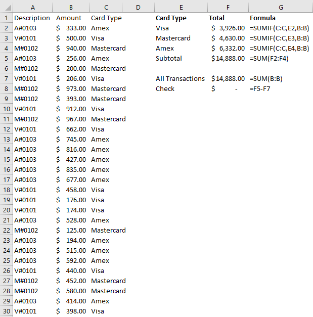
Suppose in column A you have the first letter indicating whether it’s a Visa, Mastercard, or Amex. The numbers afterward could be authorization codes. And then in column B, you have the total dollar amount of the transaction. Without the use of an array, what you might end up doing is creating another column that would use the description in column A to determine the card type. Then, you could use a SUMIF function to calculate the sales volume by card type. Here’s how that might look:

This is an approach I’d expect most people to use. It’s perfectly fine but if you’re not able to add an extra column or need to make your formula more efficient, that’s where an array can be helpful.

Through the use of an array, you don’t have to create that extra column. You can determine the card type and also sum the data all in one cell. Let’s start by calculating all the Visa transactions.

First, we’ll start by determining the card type — this process would have been the same regardless of whether you’re using an array or a SUMIF calculation. And to do this, we need to use the LEFT function to grab the first letter and determine if it is a ‘V’ to indicate Visa. This is how the formula looks like:

LEFT(A2:A30,1)=”V”

Right now, we can’t really use this on its own, it’ll just return TRUE or FALSE values. What we can do is put this formula inside of an IF function and using it as the first argument:

=IF(LEFT(A2:A30,1)=”V”

In the second IF argument, we’ll want to return the values in case the condition is true, and that V is the first character of the corresponding value in column A. In such a case, we just want to return the values that are in column B:

=IF(LEFT(A2:A30,1)=”V”,B2:B30

And if the value in column A doesn’t start with a V, then, in that case, we just want the value to be blank:

=IF(LEFT(A2:A30,1)=”V”,B2:B30,””)

I use blanks rather than a 0 value because it’s cleaner, and you’ll see why that is when I evaluate the formula further down.

The formula will now return a list of values, ignoring those which don’t start with a V in column A. All that’s left now is to sum those values. To do that, we’ll simply wrap the function above inside the SUM function and freeze the cells:

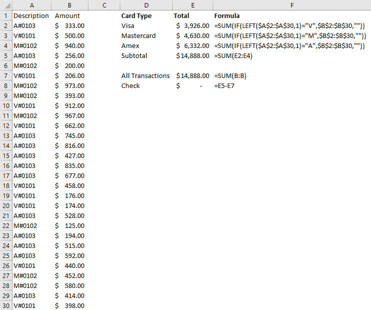
=SUM(IF(LEFT($A$2:$A$30,1)=”V”,$B$2:$B$30,””))

And here’s the result:

If you’re using an older version of Excel, you may need to use CTRL+SHIFT+ENTER to turn this into an array formula. But on newer versions, it’s no longer necessary. I didn’t need to in my case, and I can show you that it still calculates as an array. If I run the EVALUATE FORMULA button on the Formulas tab, you’ll see that it is evaluating each cell and pulling the first letter from each of the values in column A:

Then it converts that into a series of TRUE or FALSE depending on whether those values are equal to ‘V’:

And then it returns the corresponding values if they are TRUE, and “” if they are FALSE:

Notice how easy it is to separate the numbers out from the blank cells. Had I used zeros rather than blanks, it would be a bit more difficult to discern which were Visa transactions and which were not. Anytime you can hide zero values, your data is always a lot cleaner.

The last step of this formula involves just summing all the values, which gives us our total. This is a much simpler approach than having to create another column for determining the card type. You can also use this with other functions. If we wanted to get the average Visa transaction, we could just sub out the SUM function with the AVERAGE function. Arrays are very powerful and can do some incredible things.

If you liked this post on how to use an Excel array formula to do multiple calculations at once, please give this site a like on Facebook and also be sure to check out some of the many templates that we have available for download. You can also follow us on Twitter and YouTube.