CreateCustomViews

How to Use Custom Views in Excel

Did you know that you can quickly change the look of your data in Excel with Custom Views? No need for pivot tables or having to change your file’s settings and view over and over again. If you don’t use tables but frequently change the look of your file, Custom Views can save you time.

What are Custom Views?

Custom Views in Excel allow users to save specific display settings (like column widths or cell formatting) and print settings for a worksheet. This becomes especially useful when you have a single Excel sheet but require multiple ways to interpret or present the data. Rather than manually adjusting settings each time, you can quickly switch between different Custom Views.

How do Custom Views work?

Here’s how you can create Custom Views in Excel.

First, what you may want to do is create a default view with no changes applied to it. Go to the View tab and click on Custom Views.
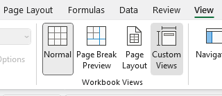
Selecting Custom Views from the View tab in Excel.

Then select Add and just call it Default.
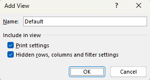
Creating a view called 'Default' in custom views.

Now, I’m going to make some changes to my data set. Here’s how it looks right now:
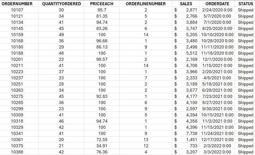
Excel data set with no changes made to it.

I’m going to apply the following changes: hide all the columns that come after Sales and filter the Quantity Ordered Field so that it only shows orders of more than 30.

Now, I’m going to repeat the steps for creating a view and this call I will call it Quantity Over 30. Now that it’s saved. I can revert back and forth between the different views. In the Custom Views page, there’s a list of the views that have been created:
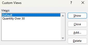
Custom views dialog box in Excel.

I can choose to Show, Add, or Delete the different views. I can also close the dialog box. If I click on Show while my Default view is selected, I’ll now get my original view, with no changes made:
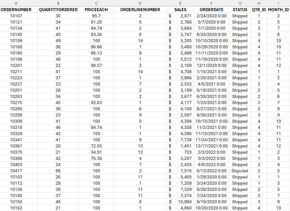
Default custom view selected in Excel.

But if I go back to my Custom Views and select Quantity Over 30, then I’ll see only a list of the orders that have more than 30 in the QuantityOrdered field. I will also no longer see those extra columns beyond Sales:
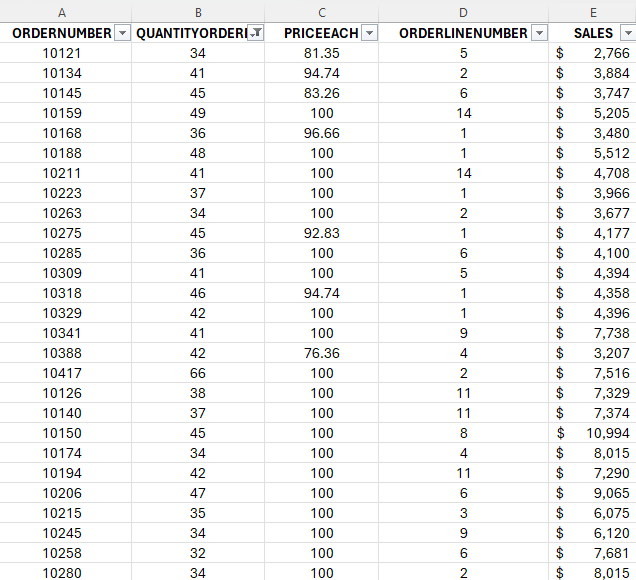
Excel sheet with the Quantity Over 30 custom view selected.

What you’ll notice is that not only have those columns been hidden, but it has also applied a filter to my data. In addition, the view will save your cell position and if you scrolled on your page. So if you happen to scroll halfway down the page and then save your view, when you go to show that view, it will do the same.

TIP: If you want to quickly access Custom Views, you can use the following shortcut: ALT+W+C. You can also right-click on the option and select Add to Quick Access Toolbar. If you do this, it’ll be added to the top of your Workbook.

When should you use Custom Views?

The biggest reason to use Custom Views is they allow you to easily filter or change the look of your data without the need for tables. This can be helpful if you’re sending the file to another user. They can just change the view and quickly see whatever they need to see. That can include filters so they only see a certain region. Or perhaps have different print settings applied so that they will work with their specific printer setup.

You can’t, however, use Custom Views if you have a table. Even if the table is on a different sheet, the Custom Views option will be unavailable. You won’t be able to use it. You may also want to avoid using Custom Views if you expect that the structure of your sheet will change. If that happens, and you haven’t created new views to reflect those changes, you may see a different view than what you expected.


If you like this post on How to Use Custom Views in Excel, please give this site a like on Facebook and also be sure to check out some of the many templates that we have available for download. You can also follow me on Twitter and YouTube. Also, please consider buying me a coffee if you find my website helpful and would like to support it.

FilterFunction

How to Use the Filter Function in Excel

Did you know that you can filter data by just using a single function in Excel? There’s no longer a need to use advanced filters or to manually select the data you want, you can just use the FILTER function, and it will give you an array of values that have met your criteria. By using the function, you can save time and make it easier to extract the data into another place on your spreadsheet.

Applying a single filter

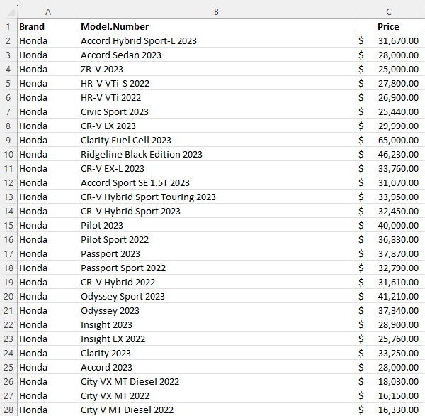
In the data set below, I have a list of makes and models of cars, and their prices.

Data set showing cars and their different prices.

Suppose you wanted to filter the data so that you only saw all the Ferraris on this list. You could use a normal filter in Excel to only see certain data. But by doing so, you will change the look of your data set. With the FILTER function, you can create a formula in another part of your spreadsheet and apply the filter you want to use.

Here’s what the formula could look like:

=FILTER(A:B,A:A=”Ferrari”)

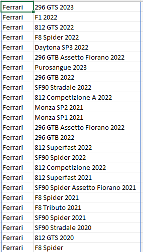
In the above formula, I’m selecting both columns A and B (brand and model.number), but I’m only filtering column A where it equals the value of Ferrari. Now, in the area where I’ve entered my formula, I get an array back of all the Ferraris, with the values that were in both A and B.

Filtered list of Ferrari vehicles.

You can apply more advanced filters than this.

Applying multiple filters

Suppose you wanted to also apply a filter so that you can see the Ferraris that are over $500,000. This part can be tricky because there’s only one argument field for what to include. The key here is to create multiple rules, and then multiply them by one another to determine if the result is true (i.e. both criteria are met).

The second criteria will be to look at column C and check if the value is more than $500,000:

C:C>=500000

To combine both of the rules, the criteria need to multiply against one another. If a criteria is met, the result is 1 (True). If it isn’t met, then it is 0 (False). So if both criteria are met, it would be multiplying 1 x 1. And if it’s a 1, then the value gets included. Here’s how the full formula looks like:

=FILTER(A:B,(A:A=”Ferrari”)*(C:C>=500000))

By deploying multiple criteria, the list of Ferraris becomes much smaller:

List of Ferrari vehicles that are more than $500,000.

You could also expand this criteria even further. To add another criteria, simply add another condition to multiply against. That way, you can have even more specific criteria to apply.

At the same time, you can use OR criteria. And this can be accomplished by adding instead of multiplying criteria. If instead of multiplying I add my criteria, now my filter will look for either a Ferrari or a car that is priced at $500,000 or over:

Vehicles that are Ferraris or that are priced at $500,000 or more.

This now covers a much broader list that includes non-Ferrari vehicles. By using multiplication and addition, you can create a variety of different rules. The key to remember is that if the end result will be a 1 (True), then it is included. If it will be a 0 (False), then it won’t be.


If you liked this post on How to Use the Filter Function in Excel, please give this site a like on Facebook and also be sure to check out some of the many templates that we have available for download. You can also follow us on Twitter and YouTube.

filterpicture1

How to Filter in Excel

If you’ve got a large data set, you know how important it is to be able to filter that data quickly and easily. Knowing how to filter efficiently in Excel can make it easy to not just pull up the data you need, but to also run calculations. Below, I’ll show you multiple ways that you can filter data.

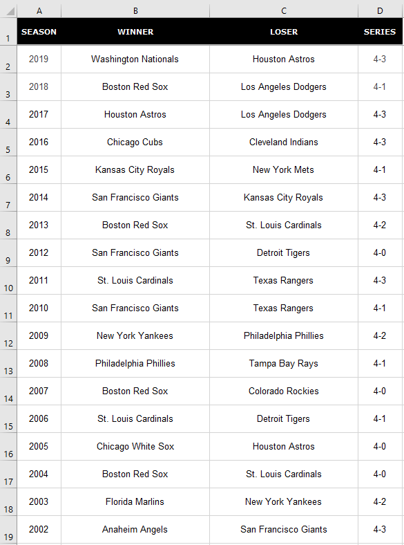
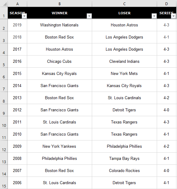
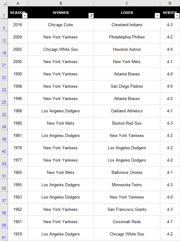
For this example, I’m going to use a list of all the MLB World Series champions and runners-up.

World Series champions and runners up.

Using the auto filter

A quick way to filter the data is by using Excel’s auto filter. To enable it, click anywhere on the data set and click on Filter button from the Data section:

Filter button on the Data tab.

Clicking the button will create drop-down buttons that you can now use to filter the data with:

Data table with filters enabled in the headers.

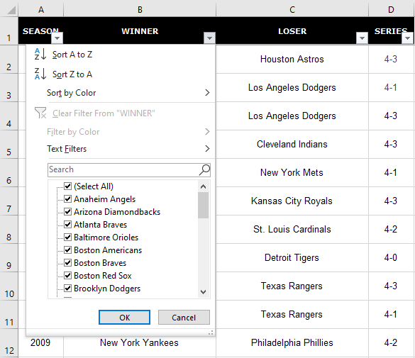
Suppose I wanted to see all the times that the New York Yankees have won. To do that, I would click on the drop-down button in the Winner column, where I’d now see all these options:

Filter options available after clicking on a drop-down.

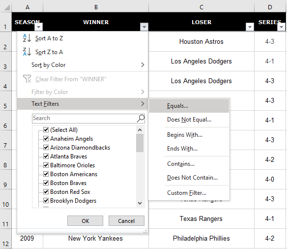
Filtering in Excel can be as easy or complicated as you want it to be. You’ll notice there’s even an option to Filter by Color that’s been greyed out since I don’t have any colors in my data set. If I click on the Text Filter option, I’ll have more options to choose from. I can look for partial matches and I can select an exact match as well:

Selecting equals as the text filter option.

In the following screen, I’ll enter in New York Yankees as my search term:

Selecting a criteria that matches only New York Yankees.

I can also have multiple criteria. For instance, I could say I want to see any victories by the New York Mets as well. In that case I could just enter another criteria and enter their name. However, there’as an even easier way to do that.

Although in the criteria, equals is selected, I can change that by clicking on the drop-down, and there I’ll have more choices:

Selecting filter criteria where the value just contains New York.

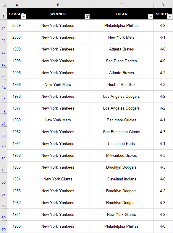
I can select contains and just change the search criteria to New York. So even though I selected equals as my initial match criteria, I don’t have to worry about sticking to it. When I click OK, I now see my list of titles won by any team that had ‘New York’ in their name:

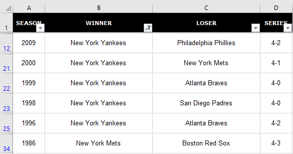
Filtered list showing any time a team from New York has won.

Not only do we have the Mets and Yankees on this list, but there’s also the New York Giants.

You’ll notice that the row numbers on the left are now in blue. This is how you can tell that your data is filtered. And so if you’re looking at your data set one day wondering why you’re missing information, have a look at the row numbers, as they may tell you the data’s filtered. If you want to unfilter the data, go back to the Filter button and click it again. Then your data set will be unfiltered and the drop-downs will be gone.

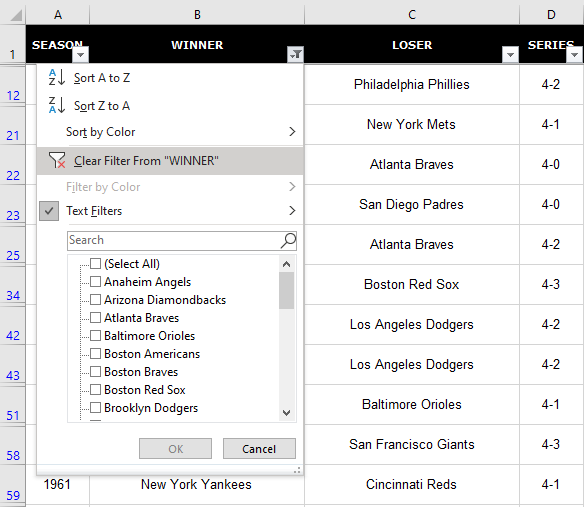
What you can also do is select the individual drop-down and clear the filter. You can tell which column has a filter in place by looking at the drop-down. In the Winner tab, the button shows a filter icon:

Drop down shows a filter icon, indicating the column has been filtered.

Clicking on that drop-down I’ll have the option to eliminate the filter:

Clearing a filter.

Clicking the Clear Filter From “WINNER” button will now reset the filter and keep the drop-down buttons in place.

Filter using selections

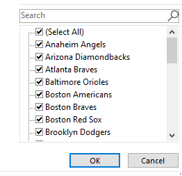
Using the text filter isn’t optimal because on newer version of Excel you see the list of items that you can choose from:

Choosing from the values list.

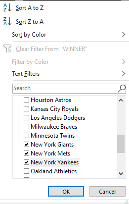
If I uncheck Select All and then scroll down to the New York teams and select them, I’ll arrive at the same result as if I did the text filter earlier:

Checking off the values to filter.

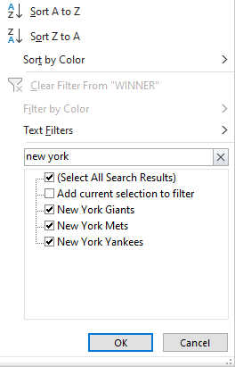
However, even this isn’t optimal. If I’m looking for a partial match, then I can just type in ‘New York’ in the search field and it’ll get the same selections:

Filtering by using the search field.

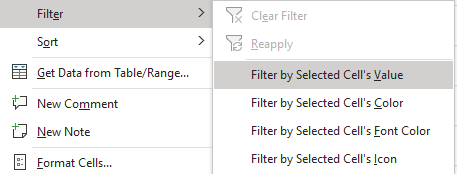
There’s another less common way that you can filter data. If you’re just looking for one match, you can right-click on the value that you want to filter. Then, right-click on it and click Filter by Cell’s Value:

Filtering by selection.

With this method, the drop-downs in the headers don’t have to be enabled. Once you run this filter, they will be there, however.

Filtering multiple combinations

It’s easy to filter when the names are similar. But if I wanted to filter the data for anytime a team from New York, Chicago, or Los Angeles has won, then it gets a bit trickier. One method would be to go back to the text filters and run multiple filters. But that’s an antiquated way of doing it. However, if you’re running an older version of Excel, that may be your only option.

If you can search through the filter, then there’s an easier way for you to do this. First, let’s go back to searching for ‘New York’ in the filter. We’ll again have all the New York teams in the list.

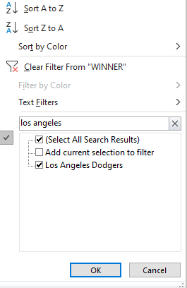
Next, let’s go back to the drop-down and search again. This time for ‘Los Angeles’ but before clicking OK, we’ll want to click off the box that says Add current selection to filter:

Add current selection to filter checkbox.

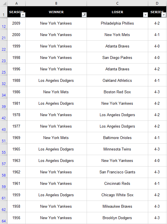
By default, this option isn’t checked. If I were to just click OK, the filter would be a list of Los Angeles teams only. But by checking off that box first and then clicking OK, I now have a list that contains both Los Angeles and New York:

Multiple cities filtered.

After repeating the process for Chicago I’ve now got all three cities in my list without having to go through the text filter:

All three cities filtered on the list.

Use subtotals to make your filters even more useful

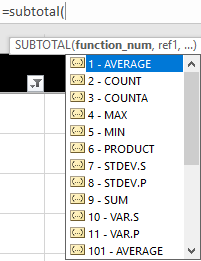
If I wanted to run a quick tally to see how many of the teams I’ve filtered have won a championship, I could use a COUNTIF function and enter their names. But if you want something more flexible where you can quickly run the filters as I’ve done above and see how many teams are in that list, you can use the SUBTOTAL function. The function takes in an argument for what type of calculation you want to do.

Arguments listed in the subtotal function.

Now, since this data isn’t numeric, I’m going to use a COUNTA function, which is function number 3. For the range, I can use any column since it doesn’t matter which one I’m counting. But I will use range A2:A1000 because I don’t want to include the header in my total. Here’s how my formula looks like:

Subtotal formula counting all the entries that have been filtered.

I could also use the MAX function to see the last time one of the teams I’ve selected has won. I’ll put that directly below the other formula:

Using multiple subtotals in a filter.

Now, if I were to re-filter this data, this time, only for New York, my subtotals will automatically update:

The benefit of using the SUBTOTAL function is your data updates along with your filters. If you want the data to be static and not change, that’s when a regular COUNTIF function would be more appropriate.


If you liked this post on how to filter in Excel, please give this site a like on Facebook and also be sure to check out some of the many templates that we have available for download. You can also follow us on Twitter and YouTube.

howtofilterdataformulas.png

Dynamically Filter Data Using Only a Formula

In my previous post I went over advanced filters in Excel. This time around I’ll go over how to achieve the same result using just a formula. No macros, no VBA, just through a not-so-simple formula that can dynamically update based on your selections.

I’m again going to use my sample database file for this example. Here’s an excerpt of what that looks like:

Filtering based on one criteria


I’m going to start by filtering all that entries for a specific sales rep.

First, I’m going to use the INDEX function to select the range from where I’m pulling data from.

=INDEX(SampleDatabase!$A$1:$G$1000

For my results, I’m going to want them to show up in the order they appear in the database. For example, in the excerpt above Rep D shows up on lines 3 and 5, and I want that same order to stay intact.

In order to do this, I’m going to use the IF, SMALL and ROW functions, which will be inserted in the INDEX function.

SMALL(IF(SampleDatabase!$C$1:$C$1000=$I$2,ROW(SampleDatabase!$A$1:$A$1000),””),ROW(A1)),1)

$C$1:$C$1000=$I$2 : In this argument, assume that $I$2 is where I have my sales rep name, in this case it would be Rep D. Because I’m only interested in rows that relate to Rep D, this is the main argument that I want to evaluate.

ROW(SampleDatabase!$A$1:$A$1000), “”) : This will return the row number if the above argument is true. It doesn’t matter whether I reference column A, B, C or any other since I’m only pulling the row number. If it isn’t a match, the result will be a blank value.

ROW(A1) : This returns a value of 1, and what this will accomplish is that it will pull the smallest row number from the above list. For instance, for Rep D we know that lines 3 and 5 will be a match, but the smallest number, or the first time that there is a match, is 3. As I drag this formula onto subsequent lines, the row number, because it isn’t frozen, will change and on line 2 it will pull the second smallest row number, on the third line it will be the third smallest, and so on.

The last argument is which column you want to extract. I left it as 1, and that will return the date since that is the first column in my INDEX argument. However, if I wanted to pull the total sales, I could change that to 7, since that would indicate column G, which is the seventh column in the data set that I specified.

The completed formula will look as follows:

=INDEX(SampleDatabase!$A$1:$G$1000,SMALL(IF(SampleDatabase!$C$1:$C$1000=$I$2,ROW(SampleDatabase!$A$1:$A$1000),””),ROW(A1)),1)

This formula will need to be entered as an array, so be sure to hit CTRL+SHIFT+ENTER.

The first five results look as follows:

The one caveat is that if you don’t know how many entries you’ll have and copy the formula down too far, you’ll inevitably end up with #NUM! errors because the formula has not found any more matches. What you can do in this case is use the IFERROR function and include it in the formula:

=IFERROR(INDEX(SampleDatabase!$A$1:$G$1000,SMALL(IF(SampleDatabase!$C$1:$C$1000=$I$2,ROW(SampleDatabase!$A$1:$A$1000),””),ROW(A1)),1),””)

What this will do is now show a blank value if there are no more matches.

Filtering for multiple criteria


While it’s nice to be able to filter for just one criteria, what if you wanted to look for the entries with multiple conditions? Although this makes our already long formula even longer, it is still possible.
Much of the formula stays the same, and the key to making it work is by changing the first argument in the IF statement. Previously, It was only looking for the Sales Rep to be a match:
$C$1:$C$1000=$I$2

I’ll add another criteria, this time for records that include Product E, and I’ll put the product criteria in the cell below in I3. I will add the following to the formula:
$D$1:$D$1000=$I$3
How I combine the two arguments is by multiplying them by one another:
($C$1:$C$1000=$I$2)*($D$1:$D$1000=$I$3)=1

I add the =1 at the end because if both conditions are true then they will result in a 1 value for that line. For example, in the first condition it will look at whether the sales rep is a match, if it is the value will be true (or 1), and if not, it will be false (or 0). The same will happen if the product matches. 
Therefore, if either one of those conditions is false then a 0 will be returned and the two conditions multiplied against one another will not equal 1.
Below is how the new formula looks:
=IFERROR(INDEX(SampleDatabase!$A$1:$G$1000,SMALL(IF(($C$1:$C$1000=$I$2)*($D$1:$D$1000=$I$3)=1,ROW(SampleDatabase!$A$1:$A$1000),””),ROW(A1)),1),””)
You’ll notice much fewer matches in column L (multiple criteria) than in column J where I was only looking for the sales rep to be a match.
If you go back to the original excerpt I showed, you’ll see that for the 3/21/2017 entry, it was for both Rep D and Product E. If I change the values in column I then my calculations will adjust accordingly.

How to Use an Advanced Filter

There are many ways you can filter data in Excel, and in this post I’ll cover the Advanced Filter.

Using the Advanced Filter will allow you to set a criteria in place for your filter and then put the results in a separate section or tab. The benefit from a normal filter where you select your criteria using drop downs is that it won’t affect the rest of the data.

If you want to follow along with my example, I have the sample database file that I’m going to use available here.

Filtering the Data Using One Criteria

First up, I’m going to look at Sales Rep A’s sales for Product A.

For the Advanced Filter to work, there are two sections that need to be ready: the criteria, and the extract.

For the criteria, you need to have the fields that you want for your filter entered. In my example I only am looking for Rep A’s Product A sales, so I only enter that criteria and don’t enter any other fields.
In the extract section, which you’ll see just below the criteria section above, I enter the fields I want to see. I don’t have to list all the fields, just the ones that I want to see. Please note the field names need to be an exact match with those in your data set. If they are not, the filter will not work as expected.
Now, to execute the Advanced Filter I’ll click on the Advanced button that is under the Data tab next to the Filter button.
After doing so, you’ll be prompted to enter two sections:

In the List range you want to enter your table, or the data you want to filter. In the Criteria Range you will select the fields you want to filter along with the criteria you want to match.

You can either Filter the list, in-place which will effectively do the same job as if you filtered your data using the drop down options. If you select Copy to another location then the third field, Copy to, will be available for input and this is where you will select your extract fields.

These are what my inputs look like:

After I click OK, my results are as follows:
This looks the same as if I were to filter using the drop down, but the benefit is I am effectively copying the data to another location.

Using Multiple Criteria

In the previous example, I used an Advanced Filter just using one set of criteria. In this example, I’ll add another to create a more complex filter. 

When using the criteria in an Advanced Filter, if criteria are on the same line it is the same as using the AND operator, while if the criteria are on different lines it is the equivalent of using OR.

In the first example, Rep A and Product A were on the same line, meaning that my criteria was that it had to be Rep A and Product A. In the following example, I’m going to add another criteria:

The above criteria says that it will look for Rep A’s Product A sales OR Product B when Total Sales are more than $500.

When I re-run the Advanced Filter, I’ll have to expand my range to include the new criteria:


The results:
The results are either Product A or B, and B only shows up when the Total Sales are more than $500. You can add even more criteria, you’ll just need to expand the criteria range when running the Advanced Filter.

Copying to Another Sheet

In both of these examples I’ve copied data over within the same tab. However, if I wanted to copy it to another sheet, that is possible as well. 
To do this, you’ll need to copy the headers you want for the extract into another tab. You need to press the Advanced Filter button on the tab where you want the data extracted to. So if you create another sheet, it’s on that sheet that you’ll need to press the button for the filter to work.
In addition to the headers, you’ll also need to put something in the second row, as the Advanced Filter button will result in an error if there is only one row of data when you click on the button (when you first use it). If there was data there before it should be fine, but the very first time you move data over you might get an error message if there isn’t data on the second row.
Once your headers are properly setup, you run the Advanced Filter button and fill in the same data as before. The one difference you’ll see is that since I’m on a different tab, the sheet name will show up in the Criteria and List range fields:

Generating a Unique List of Values

There are a lot of different ways you can pull a list of the unique values in a list. Excel has even added a button to remove duplicates, but it will remove the other items in your list, so that may not be ideal.
The Advanced Filter will allow you to do this as well, simply by just leaving your criteria blank and checking off the box for Unique records only

If I want to generate a unique list of Salespersons, I’ll run the Advanced Filter with these options:
The result:
Because I only wanted to see the unique values for the Salesperson, I only have that field in my extract list. 

Benefit of Using the Advanced Filter

At first glance, you may be wondering why even bother with an Advanced Filter. After all, you can setup the filters yourself using drop downs and then copying and pasting the filtered data somewhere else.
The most likely reason for the Advanced Filter is that in earlier versions of Excel, filtering just wasn’t as strong as it is today. 
The main benefit using it today is that it can allow you to easily audit and trace your filters. If you just copy and paste after applying filters you won’t be reminded of which filters you put in place.
If you use older versions of Excel you’ll likely find a lot more usefulness out of the Advanced Filter than if you are using the newer versions. Admittedly, I haven’t had a need to use the Advanced Filter in several years and can’t imagine that changing anytime soon.