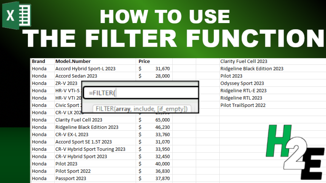
Did you know that you can filter data by just using a single function in Excel? There’s no longer a need to use advanced filters or to manually select the data you want, you can just use the FILTER function, and it will give you an array of values that have met your criteria. By using the function, you can save time and make it easier to extract the data into another place on your spreadsheet.
Applying a single filter
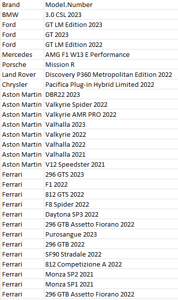
In the data set below, I have a list of makes and models of cars, and their prices.
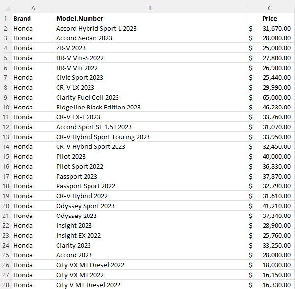
Suppose you wanted to filter the data so that you only saw all the Ferraris on this list. You could use a normal filter in Excel to only see certain data. But by doing so, you will change the look of your data set. With the FILTER function, you can create a formula in another part of your spreadsheet and apply the filter you want to use.
Here’s what the formula could look like:
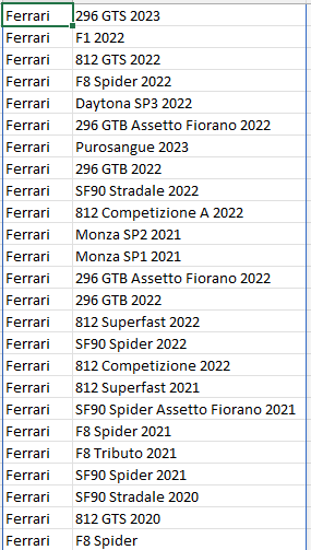
=FILTER(A:B,A:A=”Ferrari”)
In the above formula, I’m selecting both columns A and B (brand and model.number), but I’m only filtering column A where it equals the value of Ferrari. Now, in the area where I’ve entered my formula, I get an array back of all the Ferraris, with the values that were in both A and B.
You can apply more advanced filters than this.
Applying multiple filters
Suppose you wanted to also apply a filter so that you can see the Ferraris that are over $500,000. This part can be tricky because there’s only one argument field for what to include. The key here is to create multiple rules, and then multiply them by one another to determine if the result is true (i.e. both criteria are met).
The second criteria will be to look at column C and check if the value is more than $500,000:
C:C>=500000
To combine both of the rules, the criteria need to multiply against one another. If a criteria is met, the result is 1 (True). If it isn’t met, then it is 0 (False). So if both criteria are met, it would be multiplying 1 x 1. And if it’s a 1, then the value gets included. Here’s how the full formula looks like:
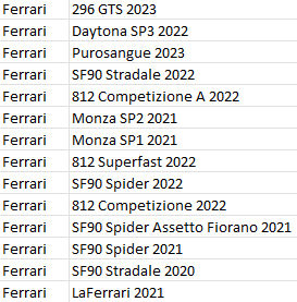
=FILTER(A:B,(A:A=”Ferrari”)*(C:C>=500000))
By deploying multiple criteria, the list of Ferraris becomes much smaller:
You could also expand this criteria even further. To add another criteria, simply add another condition to multiply against. That way, you can have even more specific criteria to apply.
At the same time, you can use OR criteria. And this can be accomplished by adding instead of multiplying criteria. If instead of multiplying I add my criteria, now my filter will look for either a Ferrari or a car that is priced at $500,000 or over:
This now covers a much broader list that includes non-Ferrari vehicles. By using multiplication and addition, you can create a variety of different rules. The key to remember is that if the end result will be a 1 (True), then it is included. If it will be a 0 (False), then it won’t be.
If you liked this post on How to Use the Filter Function in Excel, please give this site a like on Facebook and also be sure to check out some of the many templates that we have available for download. You can also follow us on Twitter and YouTube.

