Alphabet's historical stock price.

Use MAXIFS and MINIFS to Find Values Within a Range

Whether you’re using VLOOKUP or XLOOKUP, one limitation you’re going to face with those functions is that you can’t search within a range or use multiple criteria in your lookups. For example, suppose you’re looking at a stock’s history and wanted to know the last time it fell within a certain price range. You wouldn’t be able to do that with the aforementioned functions. But there is a way to accomplish that, using either MAXIFs or MINIFs. Here’s how.

Using MAXIFs and MINIFs as a lookup

With the MAXIFs and MINIFs functions, you are extracting either the smallest or largest data point in a range. And since you can apply multiple IF statements within these functions, you have the possibility to use multiple criteria. In the following example I have a list of Alphabet’s historical stock price going back multiple years:
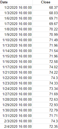
Alphabet's historical stock price.

Let’s suppose I wanted to find the last time that the stock was trading between $70 and $80. This is how the formula would look, assuming the date is in column A and the closing price is in column B:

=MAXIFS(A:A,B:B,”>=”&startprice,B:B,”<=”&endprice)

In column B, I have two criteria, one to check if the value is greater than or equal to the startprice variable ($70), and another to see if the value is less than or equal to the endprice variable ($80). Whenever that criteria is met, the value from column A is returned. And since the function is taking the maximum of those values, it will return the latest date in column A (i.e. the most recent, or the one closest to today’s date). If the date values were sorted in descending order rather than ascending order as they are above, then I would use the MINIFS function to get the same result.

Using the formula, it tells me that the last time Alphabet’s stock price was between $70 and $80 was on Oct. 29, 2020. And when looking at the range, it’s evident that looks to be correct:
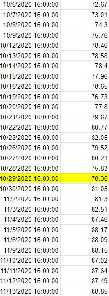
Alphabet's historical stock price.

Without the use of ranges and utilizing MAXIFS, this would have been a much more difficult process. There are multiple ways to approach a lookup and it ultimately depends on the situation and what you need to accomplish. MAXIFS and MINIFS are particularly useful when working with dates. But in other situations, you may need to use a different function instead.


If you liked this post on Use MAXIFS and MINIFS to Create a Lookup With Multiple Criteria in Excel, please give this site a like on Facebook and also be sure to check out some of the many templates that we have available for download. You can also follow us on Twitter and YouTube.

H2Esmallestnonzero

Find the Smallest Non-Zero Value in Excel

Do you need to find the smallest value but want to skip over any zero values? In this post, I’ll show you how you can do just that. The MIN function in Excel does a good job of finding the lowest value but if you have any zero values, those will get included in the result. So how can you get around the issue and get the smallest non-zero value? There are multiple ways you can accomplish this.

Using an array function

An array function allows you to evaluate each cell and that can tell the function whether to include it in its calculation. In the following example, I have a list of the numbers from 0 through to 10:

Numbers 0 through 10 are listed.

By just using the MIN function on that entire range, I will get a value of 0 as the result. However, you can get around this by embedding an IF statement within your MIN function and then turning the formula into an array. The regular MIN function would look as follows:

=MIN(A1:A11)

The IF statement will look to see if a value is not equal to 0 by using the “<>” operators:

=IF(A1:A11<>0,A1:A11)

The IF function evaluates every cell and if it’s not equal to 0, then it returns the value. Here’s how it looks embedded within the IF statement:

=MIN(IF(A1:A11<>0,A1:A11))

The result of this formula is a 1, as it will ignore any 0 values. If you’re running an older version of Excel that doesn’t calculate this correctly, you will need to use CTRL+SHIFT+ENTER to convert this into an array formula and so that you have the curly braces around it as such:

{=MIN(IF(A1:A11<>0,A1:A11))}

Using the LARGE function

Another way you can calculate the smallest non-zero number is by using the LARGE function. Technically, this is used when you want to find the largest values in a range. For instance, if I wanted to get the largest number in range A:A, my formula would be as follows:

=LARGE(A:A,1)

This is the same as if I were to use the MAX function. However, if I know there are 10 items in my range and I grab the 10th largest, that’s the same as saying I want to extract the smallest number in the range.

The key to making this work is using the COUNTIF function. With the COUNTIF, I can count the number values that are greater than zero in a range. This formula would accomplish that:

=COUNTIF(A:A,”>0″)

If I include that in my LARGE function, it will look like this:

=LARGE(A:A, COUNTIF(A:A,”>0″) )

An array calculation is not needed here since I am not evaluating every cell. And this formula arrives at the same result as the earlier method.


If you liked this post on How to Find the Smallest Non-Zero Value in Excel, please give this site a like on Facebook and also be sure to check out some of the many templates that we have available for download. You can also follow us on Twitter and YouTube.

pay-2446670_1280

Extracting the Largest and Smallest Values in a Dataset

Retrieving the maximum and minimum values is done relatively easily in Excel using the MIN() and MAX() functions, but what if you wanted to extract the five largest or smallest values?

Two lesser-known functions can help you achieve this: SMALL and LARGE. Both functions work the same way and have the same arguments: (array, k)

In the first argument (array), you select the data you want to pull your value from, and the second argument (k) is how large or small it is with respect to the data (e.g. a value of 5 would give you the fifth largest or smallest value, depending on whether you are using the LARGE or SMALL function).

You could recreate the MAX and MIN results by placing a value of 1 in the second argument, for example:

=SMALL(A:A,1) would return the smallest (minimum) value in column A
=LARGE(A:A,1) would return the largest (maximum) value in column A

However, the real value in using the SMALL and LARGE functions is being able to pull the next smallest, or largest number.

You can use the ROW() function to help you do this.

If you needed to pull the 10 largest or smallest values from a range of data, rather than manually changing the k values manually, what you can do is use the ROW() function, and use ROW(A1) in the first argument and then drag the formula down.

The relative references will change the value to A2, A3, A4, etc. Now whether you use A or B or C as the column doesn’t matter since the formula is only going to calculate the row number.

The formulas might look something like this, assuming you data is in column A:

=SMALL(A:A,ROW(A1))
=SMALL(A:A,ROW(A2))
=SMALL(A:A,ROW(A3))

The value for ROW(A1) is 1, and for ROW(A2) it is 2, so you can see how just by dragging this formula down you can easily increment your formula and pull the next largest or smallest number.

The above example would get you the three smallest values in the data set, whereas the following would return you the three largest:

=LARGE(A:A,ROW(A1))
=LARGE(A:A,ROW(A2))
=LARGE(A:A,ROW(A3))