Excel has many different functions that can help you parse out text from cells. This includes the LEN, MID, LEFT, and RIGHT functions. By utilizing these and other functions, you can get just the values you want. And by determining the number of blank spaces within a cell, you can also determine the number of words that a cell contains. There are multiple ways you can count cells in Excel, I’ll start with using the easier, and newer TEXTSPLIT function.
Method 1: Counting words using the TEXTSPLIT function
The TEXTSPLIT function is available for users who have Microsoft 365 and so if you do not see that function available as you type it in, you’ll need to move to the second approach. Using the TEXTSPLIT function, you can turn a single text value in a cell into multiple cells or columns. And you can specify how you want to split a cell; which delimiter you want to use.
In the example of counting words, the delimiter you would use is a blank space, as specified with ” ” in the delimiter argument. Here’s a list of article titles that I am going to use for this example:
The article titles are in column A. The formula to split the text every time there is a blank space would be as follows, assuming the first value is in cell A2:
=TEXTSPLIT(A2,” “)
This formula, however, would simply put all the words in different columns. Thus, it is incomplete when your goal is to count the number of words. To fix this, the formula needs to be embedded within the COUNTA function. How COUNTA works is that it simply counts the number of nonblank values.
=COUNTA(TEXTSPLIT(A2,” “))
Copying this formula down, these are the resulting values and the number of words found in each cell:
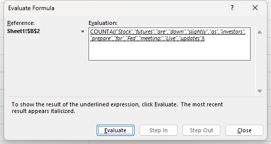
Here’s a closer look at how the formula in B2 works, using the Evaluate Formula feature in Excel:
The TEXTSPLIT function is breaking out each word as its own separate value. And the COUNTA function is then counting each one of those values. When combined, these functions allow you to count the number of words in a cell.
If you’re using Google Sheets, you can use the exact same formula as shown above, with the only difference being that instead of TEXTSPLIT, you’ll use the SPLIT function. It works in the exact same way.
Method 2: Using the LEN and SUBSTITUTE functions to count words
If you are on an older version of Excel where TEXTSPLIT isn’t available, there’s still a way that you can count the number of words within a cell. It will be a slightly more complex formula that will use the LEN and SUBSTITUTE functions.
The first part of the formula will involve counting the number of characters in a cell, which is what the LEN function does. This is accomplished through the LEN(A2) formula — assuming that A2 is where the article name is.
Next, you’ll need to use the SUBSTITUTE function to replace the blank values ” ” with an empty string that just contains two quotes: “”. To do that, the formula for that portion would be: SUBSTITUTE(A2,” “,””). This formula will need to be enclosed within a LEN function. What this accomplishes is it counts the number of characters in the cell after you’ve replaced all the blank values. If you take the total cell length and subtract this second piece, you’ll be left with the number of blank values in the text.
=LEN(A2)-LEN(SUBSTITUTE(A2,” “,””)
However, this isn’t entirely correct as you will be off by 1 word. This is because since the formula is counting the number of blanks, it won’t include the first word, which doesn’t come with a space before it. That also means if you only have one word, you’ll have a value of 0 instead of 1. To fix this, you’ll simply need to add a +1 to the end of your formula.
=LEN(A2)-LEN(SUBSTITUTE(A2,” “,””)+1
This would mean, however, that even blank cells would return a value of 1. And this would technically be the same problem when using the TEXTSPLIT function as well, since it doesn’t check for blanks, either. To correct this, you can simply add an IF function to check if the value is indeed blank. Here’s how the full formula looks:
This will return nothing if the cell is blank. If the cell isn’t blank, then it will go ahead and perform the rest of the calculation. As mentioned, this IF function can also be added to the start of the TEXTSPLIT function as well.
If you liked this post on How to Count Words in Excel, please give this site a like on Facebook and also be sure to check out some of the many templates that we have available for download. You can also follow me on Twitter and YouTube. Also, please consider buying me a coffee if you find my website helpful and would like to support it.
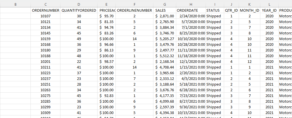
If you’re an accountant, you know that working with large amounts of data can be a daunting task. But with Excel, that work can get a whole lot easier and more efficient. Understanding Excel’s advanced features and functions can improve productivity, reduce errors, make your work more accurate, and most importantly — save you time. Below, I’ll go over some of the most important Excel functions that accountants should know, and provide examples of how to use them. For this example, I’ll use the following spreadsheet. Feel free to download it and follow along with the calculations.
1. SUM
The SUM function is a basic but essential function in Excel. It allows you to add up a range of values, which is helpful when calculating totals, such as revenue, expenses, and profits. Suppose you have a spreadsheet with sales data. In the above example, the total sales are in column G. If you wanted to sum up the entire column, the formula would be as follows: =SUM(G:G)
2. AVERAGE
The AVERAGE function calculates the average of a range of values. It is useful when analyzing data and preparing financial statements. In the above example, suppose you wanted to calculate what the average sale was. To do this, you can just use the AVERAGE function on column G, similar to the SUM function before. Here’s the formula: =AVERAGE(G:G)
3. IF
The IF function allows you to test a condition and return one value if the condition is true and another value if the condition is false. This can be useful because it can send your formulas to the next level. By knowing to use the IF function, you could also use SUMIF, AVERAGEIF, and many other functions that involve an if statement. In the above example, let’s say you only wanted to know if a value in cell M2 was part of the Motorcycles product line. The formula would be as follows: =IF(M2=”Motorcycles”,1,2). If it is part of Motorcycles, you would have a value of 1, otherwise, it would be 2.
4. SUMIF
By knowing the SUM and IF functions, you can combine them together with SUMIF, which is an incredibly popular function. It gives you a quick way to tally up the totals that meet a criteria. For example, let’s say you want all sales that relate to the Motorcycles category. The formula for that would be as follows: =SUMIF(M:M,”Motorcycles”,G:G). If the criteria is met in column M, then the formula will sum up the corresponding values in column G. There’s also the super-powered SUMIFS function, which allows you to combine multiple criteria.
5. EOMONTH
The EOMONTH function calculates the last day of the month for a specified number of months in the future or past. It is useful when working with data that is organized by date. For accountants, this can be useful when you’re calculating when something is due. Let’s say in this example, we need to calculate the date orders need to go out on, and that needs to be the end of the next month. Using the ORDERDATE field in column H, here’s how that calculation would look in the first cell, which would then be copied down for the rest: =EOMONTH(H2,1)
6. TODAY
The TODAY function is helpful for accountants in calculating deadlines and knowing how many days are remaining or past a certain date. Suppose that you wanted to know how many days have past since the ORDER DUE DATE that was calculated in the previous example. Rather than entering in a static date that every day you would need to change, you can just use the TODAY function. Here’s how a formula calculating the days since the deadline for the first cell would look like, assuming the due date is in column N: =TODAY()-N2. The next day you open up the workbook, the calculations will update to reflect the current date; there’s no need to make any changes. There are many more date calculations you can do in Excel.
7. FV
The FV function calculates the future value of an investment based on a fixed interest rate and a regular payment schedule. You can use it to calculate the future value of an investment or savings account. Let’s say that you wanted to save $10,000 per year and expect to earn a return of 5% per year on that investment. Using the FV calculation, you can do that with the following formula: =FV(0.05,5,-10000). If you don’t enter a negative for the payment amount, the formula will result in a negative value. You can also specify whether payments happen at the beginning of a period (1) or end (0 — this is the default) with the last argument in the function.
8. PV
The PV function lets you do the opposite and work backwards from a future value to the present. Knowing that the calculation in example 7 returns a value of $55,256.31, that can be used in the PV calculation to check our work: =PV(0.05,5,10000,-55256.31). The formula returns a value of 0, which is correct, as there was no starting value in the FV calculation.
9. PMT
The PMT function calculates the periodic payment required to pay off a loan with a fixed interest rate over a specified period. It is helpful when determining the monthly payments required to pay off a loan or mortgage. Let’s take the example of a mortgage payment where you need to pay down $500,000 over the period of 30 years, in monthly payments. At a 5% interest rate, here’s what the payment calculation would be: =PMT(0.05/12,12*30,-500000,0). Here again the ending value needs to be a negative to avoid a negative value in the result. And since the payments are monthly, the periods need to be multiplied by 12 and the interest rate is dividend by 12.
10. VLOOKUP
The VLOOKUP function allows you to search for a value in a table and return a corresponding value from another column in the same row. It’s one of the most common Excel functions because of how useful and easy to use it is. It is helpful when working with large data sets and performing data analysis. Let’s suppose in this example that you want to find the sales related to order number 10318. The formula for that calculation might look like this: =VLOOKUP(10318,C:G,5,FALSE). In a VLOOKUP function, you need to specify the column number you want to extract from, which is what the 5 represents. If you’re using Office 365, you can also use the newer, flashier XLOOKUP function. I put VLOOKUP on this list because it’ll work on older versions of Excel — XLOOKUP won’t.
11. INDEX
The INDEX function allows you to return a value from a data set by specifying the row and column number. It’s also helpful if you just want to return data from a single row or column. For example, the sales column is in column G. If I know the order number is on row 20 (which relates to order number 10318), this formula would do the same job as the VLOOKUP in the previous example: =INDEX(G:G,20,1).
12. MATCH
The MATCH function allows you to find the position of a value within a range of cells. Oftentimes, Excel users deploy a combination of INDEX and MATCH instead of VLOOKUP due to its limitation (e.g. VLOOKUP can’t extract values to the left of the lookup field). In the previous example, you had to specify the row belonging to the order number. But if you didn’t know it, you could use the MATCH function within the INDEX function. The MATCH function would look like this: =MATCH(10318,C:C,0). Placed within an INDEX function, it can replace the argument where in the previous example, we set a value of 20: =INDEX(G:G,MATCH(10318,C:C,0),1). By doing this, you have a more flexible version of the VLOOKUP function. You can also create dynamic formulas using INDEX and MATCH that use lookups for both the column and row.
13. COUNTIF
The COUNTIF function allows you to count the number of cells in a range that meet a specified condition. Let’s count the number of values in the data set that are Motorcycles. To do this, you would enter the following formula: =COUNTIF(M:M,”Motorcycles”).
14. COUNTA
The COUNTA function is similar to the previous function, except it only counts the number of non-empty cells. With no criteria, it is helpful to just the total number of values within a range. To calculate how many cells are in this data set, you can use the following formula: =COUNTA(C:C). If there are no gaps in data, then the result should be the same regardless of which column is used. And when combined with the UNIQUE function, you can have an easy way to count the number of unique values.
15. UNIQUE
The UNIQUE function returns a list of unique values within a range, and it’s a much easier method than the old-school way of extracting unique values. If you wanted to extract all the unique product lines in column M, you would enter the following formula: =UNIQUE(M:M). If, however, you just wanted to count the number of unique values, you could embed it within the COUNTA function as follows: =COUNTA(UNIQUE(M:M)). You can adjust your range if you don’t want to include the header.
This is just a sample of some of the useful Excel functions that accountants can utilize. If you are familiar with them, you’ll put yourself in a great position to improve the efficiency of your workflow and make your spreadsheets easier to use. Plus, you can confidently say that you are highly competent with Excel, which can make your resume more attractive and make you better suited for accounting jobs that require advanced Excel skills — and there are many of them that do!.
If you liked this post on 15 Excel Functions Accountants Should Know, please give this site a like on Facebook and also be sure to check out some of the many templates that we have available for download. You can also follow me on Twitter and YouTube. Also, please consider buying me a coffee if you find my website helpful and would like to support it.
Do you want to learn how to quickly count the number of cells that meet certain criteria? How about partial matches using wildcards? Below, I’ll show you how you can do this using the COUNTIF function in Excel along with similar tasks.
How does the COUNTIF function work?
As the name suggests, the COUNTIF function in Excel will count the values in a range if they meet certain criteria. It is not case-sensitive and in most cases, people use it for entire matches. However, you can also use it if you want partial matches.
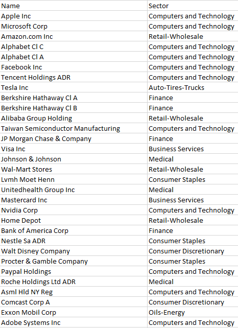
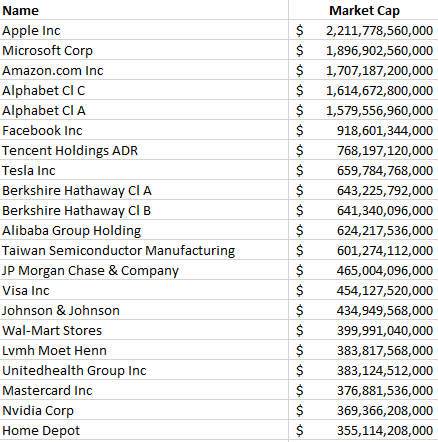
In the data sample below, I have a list of the largest stocks on the North American markets along with the sectors that they are in:
In total, my list contains 1,000 companies. To count the number that are in the Computers and Technology sector, I can do the following formula:
=COUNTIF(B:B,”computers and technology”)
Column B is where the sector name is. The above formula returns a value of 170. You’ll notice in the formula I didn’t bother matching the case because it isn’t case-sensitive and doesn’t matter how you enter the criteria in.
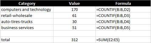
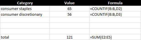
A better way to set this up is to reference an actual cell rather than hard-coding the criteria. This can help prevent errors and you don’t have to go into the cell to see what it is searching for. Here’s what the formulas look like:
I also added a SUM function at the bottom to see how many of the sectors are accounted for. With these formulas in place, I can easily copy down these functions to accommodate more sectors if I need more. This is what the COUNTIF function looks like in its simplest form. Next, let’s use wildcards to take it to the next level.
Using wildcards in a COUNTIF formula
There are two sectors in this data set that are similar — consumer discretionary and consumer staples. If I use the approach above, I would need to create COUNTIF formulas for both of them and then total them up:
This isn’t optimal and since the word ‘consumer’ is in both sectors, I can just have the COUNTIF function look for that, rather than creating two separate formulas and then a third to total them. To accomplish this, I’m going to use a wildcard to just look for the word ‘consumer’ :
=COUNTIF(B:B,”consumer*”)
You’ll notice the asterisk at the end of the word ‘consumer’ which will ensure that it will also include any text that comes after it. But how can this work to make the formula dynamic and reference a cell? To do that, I’ll use the & to connect the string to the asterisk:
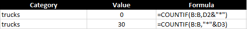
D2 is where the consumer value is, and by linking that with the asterisk (*) it still allows the cell to be dynamic. In the following example, I put the asterisk at the end of the text but you can also put it at the beginning if you want the value to end with the word:
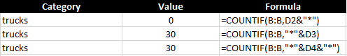
In my data, there is nothing that starts with trucks, but there are 30 values that end with it. The second formula counts those that end with the value. But what if you don’t care and just want to count every instance, regardless of where it is in the text? In that case, just add the asterisk before and after the criteria:
Suppose I just wanted to count all the sectors that included the letter ‘s’ :
A total of 709 sectors include the letter ‘s’ in their descriptions.
Using COUNTIF with blanks
You may also want to calculate how many of the cells are blank, nonblank, or don’t contain anything. Let’s cover those sections below:
Counting blanks cells
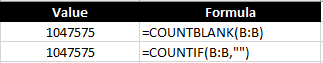
To count all the blank values you have two options. You can use the COUNTIF along with an empty string (“”) or you can use the COUNTBLANK function if it is available on your version of Excel. Both can generate the same results:
Since I’m looking at the entire column, there are many blank cells in my entire range.
Counting nonblank cells
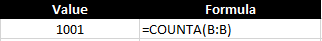
If you want to count the cells that have values in them, this is what the COUNTA function is used for:
My data set had 1,000 values in it and with the header, and so the formula returns a correct result of 1,001.
Using COUNTIF to count numbers
So far, I’ve covered how you can use the COUNTIF function in Excel with text. But you may also want to count numerical values as well. In this example, I am going to pull in the market capitalization of each of the stocks listed earlier. Here’s what that looks like:
You can use the COUNTIF function like with text but exact matches aren’t as useful when it comes to numbers. Neither are wildcards. Using the greater than (>) or less than (<) operations will be much more helpful in this situation.
Let’s start with a scenario where I want to count all the stocks that are worth more than $1 trillion. To do this, my formula looks as follows:
=COUNTIF(B:B,”>1000000000000″)
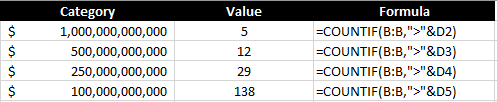
Like with the wildcard, the greater than sign goes within the quotes, as does the number. You can also connect this to a cell using the & sign to make it more dynamic:
By referencing a cell and applying a number format, it is also easier to read the value than having to rely on counting the right number of zeroes within the formula. This formula correctly returns the number 5, indicating the number of stocks on the list with valuations of more than $1 trillion. I can copy this formula down and apply it to other valuations as well:
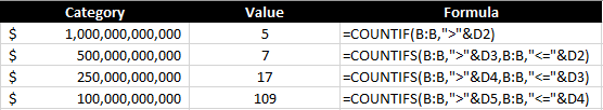
Each threshold tells me the number of stocks that are worth at least that value. But what if I don’t want to overlap and just want to know the number of companies between $500 million and $1 trillion? To do this, you will want to use the COUNTIFS function, which allows you to enter multiple criteria. It works similar to the COUNTIF function and you just continuing adding a pair of arguments (one for the range, the other for the criteria) until you are done. To count the number of companies that fall within $500 million and $1 trillion, my formula would look as follows:
In this example, I also included the equals ‘=’ operator so that it includes values that are less than or equal to $1 trillion.
This is how it might look in a table where you want the values to update dynamically:
In the first row, the COUNTIFS function isn’t needed since that is only looking at one criterion. But for the other calculations, it is pulling in only the values that fall within that range ensuring that they don’t overlap with other categories.
If you liked this post on how to use COUNTIF in Excel, please give this site a like on Facebook and also be sure to check out some of the many templates that we have available for download. You can also follow us on Twitter and YouTube.
Counting blank and non-blank cells is fairly straightforward, but what about the cells that have formulas in them that don’t return a result and look blank? They can distort those calculations. In this post, I’ll cover how to count the number of cells with text in an Excel spreadsheet (regardless of if they contain formulas or not), using multiple approaches.
I’ll use the table below for the basis of my calculations which includes some values that look empty (even though they aren’t).
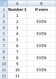
In column A I have the numbers from 1 to 11 listed. In column B I have a formula to determine if the number in column A is even, and if it is, I will place the word EVEN as my result, otherwise, it will be blank. The formula I used is the MOD function, which tells me how many remainders there are after dividing by a number. It has two arguments: the number I want to divide, and by what factor. My formula in cell B2 looks as follows:
=IF(MOD(A2,2)=0,”EVEN”,””)
In the above example, I am dividing cell A2 (1) by 2 and saying if it equals 0 (suggesting no remainder), then I want the result to return the word EVEN, otherwise, I want the cell to be blank (“”). Since 1 divided by 2 does have a remainder, the result in column B is a blank value (“”). In the next row, since the number 2 does not have a remainder, the result in column B is “EVEN.”
All the cells from B2:B12 have formulas, although some look empty.
Using COUNT, COUNTA, COUNTIF Functions
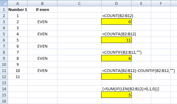
The conventional way to count non-empty cells is using the COUNTA function. A:
>=COUNTA(B2:B12)
The above formula will return a result of 11, since all 11 cells in the range are not empty, which is correct. But this doesn’t tell me how many actually contain values. If I wanted to count how many cells had numbers, I would use the COUNT function. This won’t count text, however.
=COUNT(B2:B12)
The above formula yields a result of 0, since there are no numbers in that range, otherwise, it would have worked fine. One workaround I could do is the COUNTIF function. I can count the number of blanks(“”) in the range:
=COUNTIF(B2:B12,””)
This returns a result of 6. I could combine the COUNTIF and COUNTA functions to arrive at my answer as to the number of cells that contain values that aren’t formulas:
=COUNTA(B2:B12)-COUNTIF(B2:B12,””)
This will result in 11-6 = 5. In Excel, there is usually not one way to solve a problem, so I’ll show you another way to accomplish this.
Using An Array Formula
The great thing about array formulas is they allow you to do multiple things in one formula that you couldn’t otherwise do with regular formulas (at least, not in one step). I am going to use the LEN function which tells me the length of a cell. If a cell is empty, it will return 0. If there is even one letter or digit, LEN will equal 1. I want to evaluate every cell’s length, and then tally all those that have a length of at least 1.
The LEN function would look as follows:
=LEN(B2)
This will result in a value of 0, since cell B2 has nothing in there (even though a formula exists). It is a simple function with only one argument as you can see. I will go a bit further and combine it with an IF function to return a value of 1 if there is something in the cell, and a value of 0 if there is not.
=IF(LEN(B2)>0,1,0)
The last step is to use the SUM function to now total all these values. If the non-empty cells return values of 1, then I just need to sum them all of them to get my count. The formula (before turning into an array) looks like this:
=SUM(IF(LEN(B2:B11)>0,1,0))
All I have added is the SUM function before my IF function, as well as an additional closing bracket. To turn it into an array formula, when editing the cell I have to click CTRL+SHIFT+ENTER and my formula will now look as follows (on newer versions of Excel you don’t need to do this):
{=SUM(IF(LEN(B2:B12)>0,1,0))}
This will return a result of 5 which correctly returns the same result as when I combined the COUNTA and COUNTIF functions. Below is a summary of the results:
If you liked this post on How to Count the Number of Cells With Text in Excel, please give this site a like on Facebook and also be sure to check out some of the many templates that we have available for download. You can also follow us on Twitter and YouTube.