How to Use the New XLOOKUP Function

Forget using VLOOKUP or even INDEX and MATCH, Excel users can now use XLOOKUP!

Knowing how to use VLOOKUP has become almost a basic skill for Excel users. If you’re an intermediate or advanced user, you probably use INDEX & MATCH because of the limitations that are inherent with just using VLOOKUP. Since VLOOKUP can only return values to the right of what the value that you’ve found, it’s a less-than-optimal formula. You can either re-arrange your data, or you can use INDEX & MATCH. It’s a more flexible solution, but it’s also not ideal. After all, you’re now combining multiple Excel functions into one.

Enter: XLOOKUP

XLOOKUP is the solution that Excel users have been looking for…for decades. What the function does is allow you to do what was possible with INDEX & MATCH all in one simple formula.

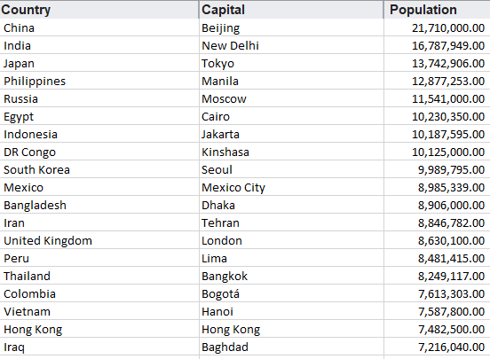
Let’s go over it with some sample data on the world’s largest cities:

Doing a regular lookup vs XLOOKUP

Here’s how my formulas would look like if I wanted to return the Country using a value from the City field:

In the above example, E5 refers to the capital city value. While the INDEX & MATCH combination works, it may not be the easiest for novice users who aren’t comfortable with nesting functions. Here’s how the same calculation would look using XLOOKUP:

It’s a much simpler solution. The first argument takes the value you want to look for, followed by the range where you want to search for it, and then the range that you want to extract the corresponding value from. There’s no need to enter a column number the way you do with VLOOKUP, nor is there a need to add another function.

There are optional arguments you can use including how you want to match (see the next section). You can also choose the direction that the lookup goes, in case you don’t want to look in the same order as your data:

Using wildcards in XLOOKUP

Like with the other functions, you can also incorporate wildcards into XLOOKUP as well. Wildcards work similarly among all three formulas, but the key difference is that XLOOKUP has multiple arguments for its fourth (optional) argument which dictates how you want the data extracted. Entering ‘2’ will tell the function that you want to use a wildcard. Below are the options for the match_mode argument (optional):

• 0: exact match
• -1: exact match or next smaller item
• 1: exact match or next larger item
• 2: wildcard character match

Here’s a comparison of how you’d get the same result using all three functions using a wildcard:

The logic is the same in the sense that you’ll want to use a wildcard character like * around the term you’re trying to find a match of. In the above example, I used the * around the entire wildcard, and it returned the population for New Delhi in that example.

XLOOKUP here is actually a bit more complicated as with the other functions you didn’t need to specify that you were using a wildcard. Taking out the ‘2’ from the argument would result in XLOOKUP yielding an #N/A error. However, it could be that doing this will make it more efficient.

Finding the closest matches

One of the other options for the matches mentioned above were finding the next smaller or next larger matching items if an exact one wasn’t found. A good example of this is where you’re looking for something like a tax rate where you won’t find every possible income level that someone might enter and you need to ensure that it falls into the correct range.

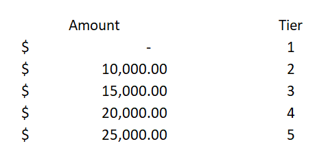
Here are some sample categories:

If I entered an amount of $17,000, it should put me in Tier 3, since that would be the threshold I would have reached under this hierarchy. Here’s an example of how this would be calculated in the three functions:

All three formulas were able to return the same tier correctly, however, INDEX & MATCH is a bit more cumbersome again due to having multiple functions within it.

The advantage that XLOOKUP has here is that I can select the category that’s either directly below or above the amount I enter, effectively rounding up or down, simply by changing the fourth argument between a ‘1’ (exact or next largest item) to a ‘-1’ (exact or next smallest item).

This is not possible with VLOOKUP, and in order for this to be able to work with INDEX & MATCH, I’d have to change the order from ascending to descending. But what’s impressive is that XLOOKUP is able to find the correct category even if the values are not in any sort of order at all.

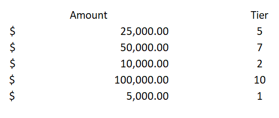
Have a look at what happens when I try to completely destroy any sort of hierarchy:

This is an absolutely dreadful hierarchy that’s not consistent in any way possible. Do the formulas have any chance of getting it right? Here’s how the results looked:

Both the INDEX & MATCH as well as the XLOOKUP formulas were looking for the closest matches. INDEX & MATCH returned the lowest tier, which technically was incorrect since $17,000 came in higher than $10,000, which was Tier 2. And XLOOKUP, despite the mess of a hierarchy, was still able to pull out the correct group.

Ultimately, you never want to organize your data in such a horrible way, but this helps demonstrate just how strong XLOOKUP is, to be able to still come out with the correct calculation.

And just for fun, let’s flip the formulas around, this time looking for an exact match or the next largest category:

There wasn’t a Tier 3 in my incomplete table, but XLOOKUP still found the next largest Tier which was at $25,000 – Tier 5. INDEX & Match found its way into Tier 7.

Creating a dynamic formula

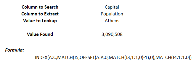
One of the great things about INDEX & MATCH is that you can index an entire database and then dynamically change which column you want to extract from based on a selection and not have to update the range in the formula. For example:

Why would you want to do this? The beauty of it is that you can change what value you extract based on your selection. Since you’re doing a match, it will look for that field and adjust the column accordingly using the OFFSET function:

You can do this in XLOOKUP as well, and here’s how that formula would compare to index and match:

The XLOOKUP formula is a bit more complicated as it needs two ranges, and thus, two OFFSET functions are needed. In the INDEX & MATCH combination, only one OFFSET function is needed as it only requires a column number for one of its arguments. Either way, you still need to be familiar with using OFFSET so it’s probably not a dealbreaker if XLOOKUP is a bit longer.

Great, so how do I get XLOOKUP?

There are two things you need to be able to get access to XLOOKUP:

• Office 365
• Enrollment in the Office 365 Insiders Program

It’s not an exclusive club or anything, all you have to do is to follow the steps outlined here. By selecting the ‘Insider’ option rather than Monthly, you’ll get more frequent updates and changes. Once you’ve got it set up, then it’s just a matter of waiting for the updates to roll out to you. There’s, unfortunately, no notification, I’d just suggest checking every now and then to see if XLOOKUP shows up in your functions list.

Caveat

One of the things you should remember, however, is that while it may be great to use XLOOKUP, old versions of Excel won’t have access to this flashy new function. And so it’s important to still be familiar with using VLOOKUP and INDEX and MATCH.

If you liked this post on How to Use the New XLOOKUP Function, please give the site a like on Facebook. Also be sure to check out our templates section. You can also follow us on Twitter and YouTube.