Creating Dynamic Formulas With Index & Match

When you create a formula in Excel, your goal should always be to minimize how much you hardcode of it. By doing that, you can make your formula more dynamic and easy to update, without having to change it. Below, I’m going to show you can create dynamic formulas in Excel, using a combination of INDEX & MATCH as an example.

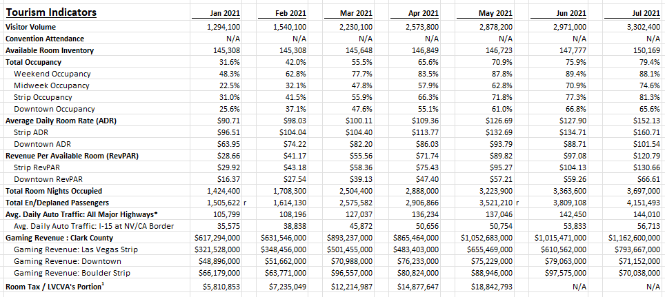
For this, I’m going to use Las Vegas visitor statistics. The goal is going to be to pull in certain values based on the combination of field and month. Here’s how the Excel download looks like to start with:

If I wanted to use lookup the visitor volume for a given month, I could use the following formula (assume the data above is in columns A:N):

=INDEX(B:B,MATCH(“Visitor Volume”,A:A,0),1)

Column B is where the January data is. And in column A, where the fields are, I’m searching for ‘Visitor Volume’. My formula returns a value of 1,294,100. That is the correct result. However, the way the formula is set up right now isn’t flexible; I hardcoded the field I was looking for and I also indicated which column I wanted to pull the results from. Ideally, I should be able to have the field set up to be dynamic, and the date as well.

Using a named range for the field

I’ll begin by making the field dynamic. Rather than type in ‘Visitor Volume’, I can just reference a named range, as such:

In the above example, I entered the field I wanted to lookup and created a named range for it, called ‘lookupfield’. Now, I can just reference the lookupfield. And if I change its value to another field, it will return a different value, all without needing to change the formula itself:

The only thing that changed here was the value I was looking up.

Using a named range for the month

Next up, I’ll adjust the formula so that the month I’ll return values from is also dynamic. This part is a bit trickier because I need to actually move the entire column. In the current formula, I’m referencing column B (which relates to the January values). But if I want to get the values for February, then it needs to change to column D, and to column F if I want March’s data, and so on.

Using the OFFSET function can be useful here. Rather than picking a specific range, I just start with the first column (A). The second argument in the OFFSET function pertains to the number of rows to move. Since I don’t want to my move my range up or down, I leave this as 0. The next argument is the number of columns I want to move. This is going to depend on where the month value is. Here again, I’ll create a named range. This time, I’ll call it ‘lookupmonth’, where I will specify the month I want to look at. In this spreadsheet, the months are just the first days of the month (e.g. Jan 2021 is 1/1/2021). I will need to use the MATCH function again, this time searching for this value within the row that contains the months (this is row 7 in my Excel sheet). Here’s what my formula will look like, fully dynamic:

=INDEX(OFFSET(A:A,0,MATCH(lookupmonth,7:7,0)-1),MATCH(lookupfield,A:A,0),1)

I add the -1 at the end of the columns argument because I’m already starting at the first column and it should be removed from the number of columns I want to move to the right. Here’s how the formula looks like with the two named ranges (highlighted in yellow):

Now, I can change both the field and the month, and my formula will automatically update:

The important thing to note here is that the named ranges need to be exact matches for the MATCH functions to work properly. Even an extra space will result in the formula not returning the correct value. One thing you may want to consider is creating a drop-down list for the available options to prevent the chance of someone making a typo and entering an invalid option.

If you liked this post on Creating Dynamic Formulas With Index & Match, please give this site a like on Facebook and also be sure to check out some of the many templates that we have available for download. You can also follow us on Twitter and YouTube.