How to Import Financial Statements Using Power Query

In this post, I’ll show you how you can import a company’s financial statements into Excel using Power Query. Previously, I’ve covered how to get stock prices from both Yahoo Finance and Google Sheets. But to get financial statement information, I’m going to use a different source: wsj.com. The reason being, is it’s in an easy format to export and that makes the import process very easy for Power Query.

Downloading the data

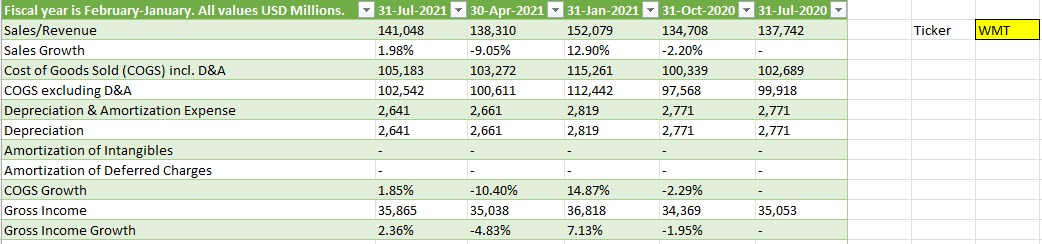
I’m going to use Walmart’s financials for this example. And if you navigate to the following URL, you will get a summary of Walmart’s quarterly financial statements:

https://www.wsj.com/market-data/quotes/WMT/financials/quarter/income-statement

What’s convenient about this URL is that it contains both the ticker, the statement type, and indicates that the financials are quarterly. That makes it easy to alter in case you wanted to look for annual statements or a balance sheet rather than an income statement. Just changing the URL will get you to the right page. The above link is what I’m going to use for this example.

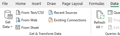
To load the data into Power Query, go to the Data tab and click on From Web:

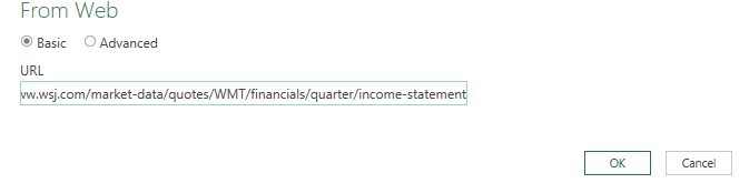
Then, paste the URL in the following box:

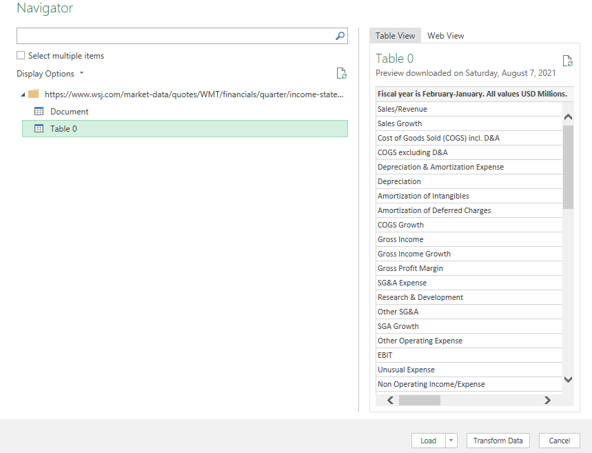
After clicking OK, you can select which table to import. In this case, it’s going to be Table 0:

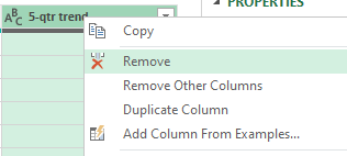
Next, press the Transform Data button to make changes before it gets imported. I’ll start with removing the column at the very end, showing the trend, as it doesn’t contain any information. To remove it, right-click on the header and click Remove:

I’m also going to remove the Changed Type step, which automatically changes the data types. To get rid of the step, click on the X next to the step:

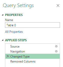
This is important because since the header names change based on the quarter, it isn’t going to be helpful to have this step since it looks for hardcoded values. An optional step you could take is to Demote Headers so that the header names are generic and not tied to a specific quarter. However, this isn’t necessary if you remove the Changed Type step. For more information on changing header names, refer to this post.

Once you’re done making changes, click on Close & Load in the top-left corner, and then your data will load into a sheet.

The download will work just fine right now. However, let’s also make the file a bit more versatile in case you want to quickly change the ticker symbol.

Setting up the variables

First up, I’ll create a named range for the ticker symbol, called ‘Ticker’ :

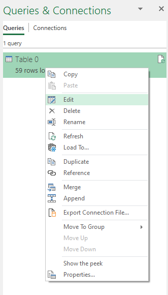
I’ll now go back into the query editor to account for this named range. To edit a query, go into the Data tab, click on Queries and Connections, and then off to the right you should see your queries. Right-click edit on the one you want to adjust:

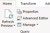
Then, click on the Advanced Editor button near the top of the Power Query window:

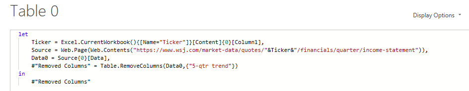
I’m going to add the Ticker variable under the let section as follows:

Ticker = Excel.CurrentWorkbook(){[Name=”Ticker”]}[Content]{0}[Column1],

Note that Power Query is case-sensitive and you will get an error if what you’ve entered doesn’t match exactly what you’ve set as your named range. Also, make sure to add a comma at the end.

I will also need to adjust the Source variable so that it uses the Ticker variable:

Source = Web.Page(Web.Contents(“https://www.wsj.com/market-data/quotes/”&Ticker&”/financials/quarter/income-statement”)),

The key thing here is to break up the part of the URL that mentions WMT and replace it with the named range. Here’s what the code looks like within the Advanced Editor:

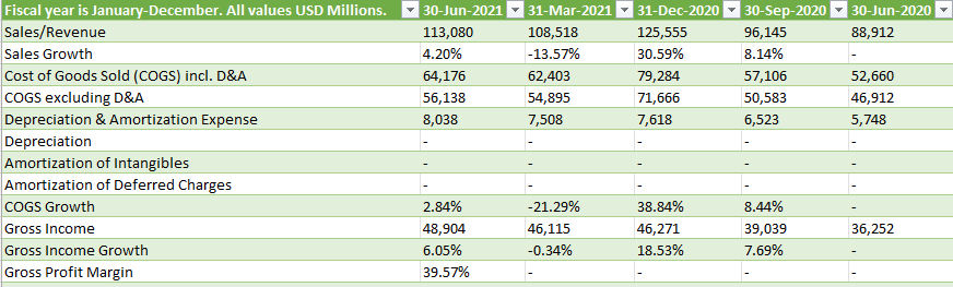
Now, you can Close & Load back into the worksheet. To test the named range, what you can do is replace the ticker value from WMT to AMZN, and if it works correctly, it should load Amazon’s income statement instead. After changing the ticker symbol, remember to press the Refresh All button under the Data tab:

If it works, you should see a whole new set of data populate on your spreadsheet:

If you liked this post on How to Import Financial Statements Using Power Query, please give this site a like on Facebook and also be sure to check out some of the many templates that we have available for download. You can also follow us on Twitter and YouTube.