How to Make a Checklist in Excel

There are many different apps to choose from if you want to create a checklist. But if you’re doing Excel work and have tasks associated with it, it may be easier to just include the checklist right within your spreadsheet. In this post, I’ll show you how you can make a checklist in Excel quickly and easily that you can re-use in many spreadsheets.

Step 1: Creating your list

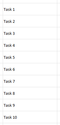
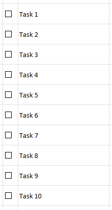
Excel is an easy place to create a list since a spreadsheet is already in a grid format. You can use either numbers or letters as prefixes, or without anything at all:

Step 2: Add checkboxes

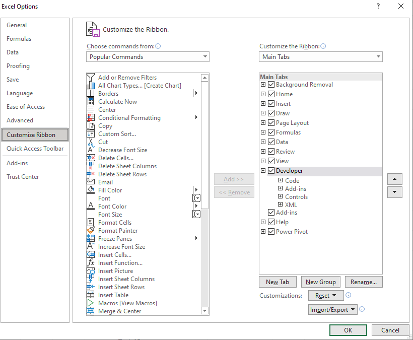
In order for this to look like a task list, we should add some checkboxes. If you don’t have the Developer tab enabled in Excel, make sure to do so. Under Excel Options, you’ll have an option to customize the Ribbon. This is where you can select which tabs you want to have enabled:

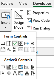
Once enabled, go to the Developer tab and click on the Insert button. Select the checkbox icon that is under the Form Controls section:

Then, use the mouse to drag and create a checkbox. It will automatically create some generic text to say ‘Check Box 1’ — you can remove this as it is unnecessary. Once you’ve got the checkbox in the position you want (and within its own cell), copy the entire cell and paste it over so that you have a checkbox next to each task:

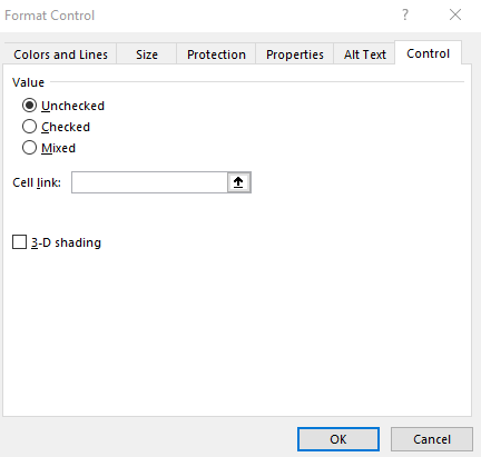
Each checkbox can be linked to a specific cell. And every time you click the checkbox, the value of that cell will toggle between TRUE and FALSE, to indicate if the box is ticked or not. To create a link, right-click on a checkbox and select Format Control. Then, under the Control section, select a cell in the Cell Link section:

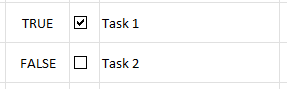
Then, when the checkbox is ticked or unticked, here’s how the values in the will appear in the linked cell:

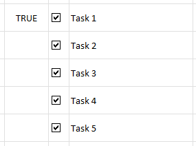
The danger with copying these checkboxes after you have linked a cell, is that those cell links won’t change; multiple checkboxes will be linked to the same cell:

To correct this, you will need to modify the cell link for each checkbox. Once that’s done, it’s time to move on to the last step.

Step 3: Add conditional formatting

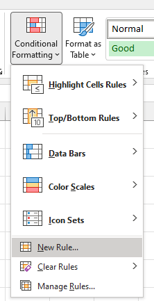
Right now, ticking the checkbox doesn’t do anything but show a TRUE or FALSE value. In this step, I’m going to add some conditional formatting to also cross out the item. To do this, I’m going to highlight the column that has the tasks (column B) and create some conditional formatting rules:

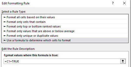
I’m going to create a rule that looks at the column that contains the cell link values (column C). It will check if the value is set to TRUE using the following formula:

=C1=TRUE

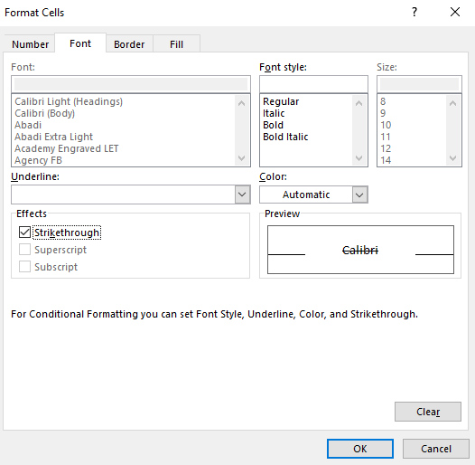
Then, under the Format options, I will apply a strikethrough effect:

Now, when a checkbox is ticked, the text will have a strikethrough effect:

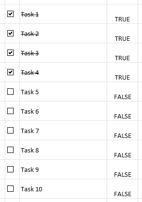
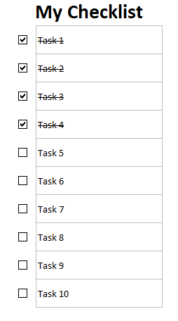
The TRUE/FALSE values can be hidden since they don’t need to be visible in order for the checkboxes and strikethrough effects to work. The only other changes you may want to make at this point relate to formatting. This includes applying a header. Here’s what your finished checklist might look like with some additional formatting:

If you liked this post on How to Make a Checklist in Excel, please give this site a like on Facebook and also be sure to check out some of the many templates that we have available for download. You can also follow us on Twitter and YouTube.