How to Use COUNTIF in Excel

Do you want to learn how to quickly count the number of cells that meet certain criteria? How about partial matches using wildcards? Below, I’ll show you how you can do this using the COUNTIF function in Excel along with similar tasks.

How does the COUNTIF function work?

As the name suggests, the COUNTIF function in Excel will count the values in a range if they meet certain criteria. It is not case-sensitive and in most cases, people use it for entire matches. However, you can also use it if you want partial matches.

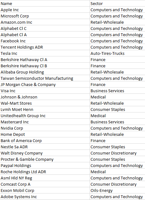
In the data sample below, I have a list of the largest stocks on the North American markets along with the sectors that they are in:

In total, my list contains 1,000 companies. To count the number that are in the Computers and Technology sector, I can do the following formula:

=COUNTIF(B:B,”computers and technology”)

Column B is where the sector name is. The above formula returns a value of 170. You’ll notice in the formula I didn’t bother matching the case because it isn’t case-sensitive and doesn’t matter how you enter the criteria in.

A better way to set this up is to reference an actual cell rather than hard-coding the criteria. This can help prevent errors and you don’t have to go into the cell to see what it is searching for. Here’s what the formulas look like:

I also added a SUM function at the bottom to see how many of the sectors are accounted for. With these formulas in place, I can easily copy down these functions to accommodate more sectors if I need more. This is what the COUNTIF function looks like in its simplest form. Next, let’s use wildcards to take it to the next level.

Using wildcards in a COUNTIF formula

There are two sectors in this data set that are similar — consumer discretionary and consumer staples. If I use the approach above, I would need to create COUNTIF formulas for both of them and then total them up:

This isn’t optimal and since the word ‘consumer’ is in both sectors, I can just have the COUNTIF function look for that, rather than creating two separate formulas and then a third to total them. To accomplish this, I’m going to use a wildcard to just look for the word ‘consumer’ :

=COUNTIF(B:B,”consumer*”)

You’ll notice the asterisk at the end of the word ‘consumer’ which will ensure that it will also include any text that comes after it. But how can this work to make the formula dynamic and reference a cell? To do that, I’ll use the & to connect the string to the asterisk:

D2 is where the consumer value is, and by linking that with the asterisk (*) it still allows the cell to be dynamic. In the following example, I put the asterisk at the end of the text but you can also put it at the beginning if you want the value to end with the word:

In my data, there is nothing that starts with trucks, but there are 30 values that end with it. The second formula counts those that end with the value. But what if you don’t care and just want to count every instance, regardless of where it is in the text? In that case, just add the asterisk before and after the criteria:

Suppose I just wanted to count all the sectors that included the letter ‘s’ :

A total of 709 sectors include the letter ‘s’ in their descriptions.

Using COUNTIF with blanks

You may also want to calculate how many of the cells are blank, nonblank, or don’t contain anything. Let’s cover those sections below:

Counting blanks cells

To count all the blank values you have two options. You can use the COUNTIF along with an empty string (“”) or you can use the COUNTBLANK function if it is available on your version of Excel. Both can generate the same results:

Since I’m looking at the entire column, there are many blank cells in my entire range.

Counting nonblank cells

If you want to count the cells that have values in them, this is what the COUNTA function is used for:

My data set had 1,000 values in it and with the header, and so the formula returns a correct result of 1,001.

Using COUNTIF to count numbers

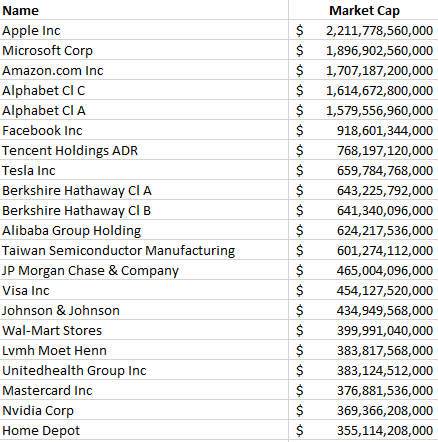
So far, I’ve covered how you can use the COUNTIF function in Excel with text. But you may also want to count numerical values as well. In this example, I am going to pull in the market capitalization of each of the stocks listed earlier. Here’s what that looks like:

You can use the COUNTIF function like with text but exact matches aren’t as useful when it comes to numbers. Neither are wildcards. Using the greater than (>) or less than (<) operations will be much more helpful in this situation.

Let’s start with a scenario where I want to count all the stocks that are worth more than $1 trillion. To do this, my formula looks as follows:

=COUNTIF(B:B,”>1000000000000″)

Like with the wildcard, the greater than sign goes within the quotes, as does the number. You can also connect this to a cell using the & sign to make it more dynamic:

By referencing a cell and applying a number format, it is also easier to read the value than having to rely on counting the right number of zeroes within the formula. This formula correctly returns the number 5, indicating the number of stocks on the list with valuations of more than $1 trillion. I can copy this formula down and apply it to other valuations as well:

Each threshold tells me the number of stocks that are worth at least that value. But what if I don’t want to overlap and just want to know the number of companies between $500 million and $1 trillion? To do this, you will want to use the COUNTIFS function, which allows you to enter multiple criteria. It works similar to the COUNTIF function and you just continuing adding a pair of arguments (one for the range, the other for the criteria) until you are done. To count the number of companies that fall within $500 million and $1 trillion, my formula would look as follows:

=COUNTIFS(B:B,”>500000000000″,B:B,”<=1000000000000″)

In this example, I also included the equals ‘=’ operator so that it includes values that are less than or equal to $1 trillion.

This is how it might look in a table where you want the values to update dynamically:

In the first row, the COUNTIFS function isn’t needed since that is only looking at one criterion. But for the other calculations, it is pulling in only the values that fall within that range ensuring that they don’t overlap with other categories.

If you liked this post on how to use COUNTIF in Excel, please give this site a like on Facebook and also be sure to check out some of the many templates that we have available for download. You can also follow us on Twitter and YouTube.