CountWords

How to Count Words in Excel

Excel has many different functions that can help you parse out text from cells. This includes the LEN, MID, LEFT, and RIGHT functions. By utilizing these and other functions, you can get just the values you want. And by determining the number of blank spaces within a cell, you can also determine the number of words that a cell contains. There are multiple ways you can count cells in Excel, I’ll start with using the easier, and newer TEXTSPLIT function.

Method 1: Counting words using the TEXTSPLIT function

The TEXTSPLIT function is available for users who have Microsoft 365 and so if you do not see that function available as you type it in, you’ll need to move to the second approach. Using the TEXTSPLIT function, you can turn a single text value in a cell into multiple cells or columns. And you can specify how you want to split a cell; which delimiter you want to use.

In the example of counting words, the delimiter you would use is a blank space, as specified with ” ” in the delimiter argument. Here’s a list of article titles that I am going to use for this example:

List of article titles in an Excel spreadsheet.

The article titles are in column A. The formula to split the text every time there is a blank space would be as follows, assuming the first value is in cell A2:

=TEXTSPLIT(A2,” “)

This formula, however, would simply put all the words in different columns. Thus, it is incomplete when your goal is to count the number of words. To fix this, the formula needs to be embedded within the COUNTA function. How COUNTA works is that it simply counts the number of nonblank values.

=COUNTA(TEXTSPLIT(A2,” “))

Copying this formula down, these are the resulting values and the number of words found in each cell:

List of article names in Excel with a corresponding number of words found.

Here’s a closer look at how the formula in B2 works, using the Evaluate Formula feature in Excel:
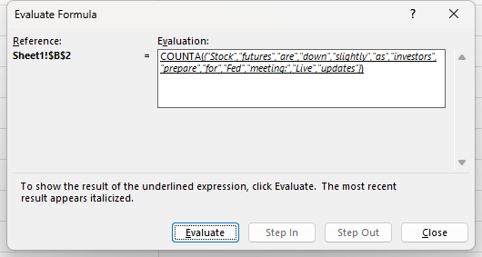
Using the evaluate formula feature in Excel to determine the number of words within a cell.

The TEXTSPLIT function is breaking out each word as its own separate value. And the COUNTA function is then counting each one of those values. When combined, these functions allow you to count the number of words in a cell.

If you’re using Google Sheets, you can use the exact same formula as shown above, with the only difference being that instead of TEXTSPLIT, you’ll use the SPLIT function. It works in the exact same way.

Method 2: Using the LEN and SUBSTITUTE functions to count words

If you are on an older version of Excel where TEXTSPLIT isn’t available, there’s still a way that you can count the number of words within a cell. It will be a slightly more complex formula that will use the LEN and SUBSTITUTE functions.

The first part of the formula will involve counting the number of characters in a cell, which is what the LEN function does. This is accomplished through the LEN(A2) formula — assuming that A2 is where the article name is.

Next, you’ll need to use the SUBSTITUTE function to replace the blank values ” ” with an empty string that just contains two quotes: “”. To do that, the formula for that portion would be: SUBSTITUTE(A2,” “,””). This formula will need to be enclosed within a LEN function. What this accomplishes is it counts the number of characters in the cell after you’ve replaced all the blank values. If you take the total cell length and subtract this second piece, you’ll be left with the number of blank values in the text.

=LEN(A2)-LEN(SUBSTITUTE(A2,” “,””)

However, this isn’t entirely correct as you will be off by 1 word. This is because since the formula is counting the number of blanks, it won’t include the first word, which doesn’t come with a space before it. That also means if you only have one word, you’ll have a value of 0 instead of 1. To fix this, you’ll simply need to add a +1 to the end of your formula.

=LEN(A2)-LEN(SUBSTITUTE(A2,” “,””)+1

This would mean, however, that even blank cells would return a value of 1. And this would technically be the same problem when using the TEXTSPLIT function as well, since it doesn’t check for blanks, either. To correct this, you can simply add an IF function to check if the value is indeed blank. Here’s how the full formula looks:

=IF(A2=””,””,LEN(A2)-LEN(SUBSTITUTE(A2,” “,””))+1)

This will return nothing if the cell is blank. If the cell isn’t blank, then it will go ahead and perform the rest of the calculation. As mentioned, this IF function can also be added to the start of the TEXTSPLIT function as well.


If you liked this post on How to Count Words in Excel, please give this site a like on Facebook and also be sure to check out some of the many templates that we have available for download. You can also follow me on Twitter and YouTube. Also, please consider buying me a coffee if you find my website helpful and would like to support it.

Table containing numbers specifying if they are even or not.

How to Count the Number of Cells With Text in Excel

Counting blank and non-blank cells is fairly straightforward, but what about the cells that have formulas in them that don’t return a result and look blank? They can distort those calculations. In this post, I’ll cover how to count the number of cells with text in an Excel spreadsheet (regardless of if they contain formulas or not), using multiple approaches.

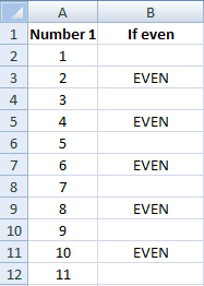
I’ll use the table below for the basis of my calculations which includes some values that look empty (even though they aren’t).

Table containing numbers specifying if they are even or not.

In column A I have the numbers from 1 to 11 listed. In column B I have a formula to determine if the number in column A is even, and if it is, I will place the word EVEN as my result, otherwise, it will be blank. The formula I used is the MOD function, which tells me how many remainders there are after dividing by a number. It has two arguments: the number I want to divide, and by what factor. My formula in cell B2 looks as follows:

=IF(MOD(A2,2)=0,”EVEN”,””)

In the above example, I am dividing cell A2 (1) by 2 and saying if it equals 0 (suggesting no remainder), then I want the result to return the word EVEN, otherwise, I want the cell to be blank (“”). Since 1 divided by 2 does have a remainder, the result in column B is a blank value (“”). In the next row, since the number 2 does not have a remainder, the result in column B is “EVEN.”

All the cells from B2:B12 have formulas, although some look empty.

Using COUNT, COUNTA, COUNTIF Functions

The conventional way to count non-empty cells is using the COUNTA function. A:

>=COUNTA(B2:B12)

The above formula will return a result of 11, since all 11 cells in the range are not empty, which is correct. But this doesn’t tell me how many actually contain values. If I wanted to count how many cells had numbers, I would use the COUNT function. This won’t count text, however.

=COUNT(B2:B12)

The above formula yields a result of 0, since there are no numbers in that range, otherwise, it would have worked fine. One workaround I could do is the COUNTIF function. I can count the number of blanks(“”) in the range:

=COUNTIF(B2:B12,””)

This returns a result of 6. I could combine the COUNTIF and COUNTA functions to arrive at my answer as to the number of cells that contain values that aren’t formulas:

=COUNTA(B2:B12)-COUNTIF(B2:B12,””)

This will result in 11-6 = 5. In Excel, there is usually not one way to solve a problem, so I’ll show you another way to accomplish this.

Using An Array Formula

The great thing about array formulas is they allow you to do multiple things in one formula that you couldn’t otherwise do with regular formulas (at least, not in one step). I am going to use the LEN function which tells me the length of a cell. If a cell is empty, it will return 0. If there is even one letter or digit, LEN will equal 1. I want to evaluate every cell’s length, and then tally all those that have a length of at least 1.

The LEN function would look as follows:

=LEN(B2)

This will result in a value of 0, since cell B2 has nothing in there (even though a formula exists). It is a simple function with only one argument as you can see. I will go a bit further and combine it with an IF function to return a value of 1 if there is something in the cell, and a value of 0 if there is not.

=IF(LEN(B2)>0,1,0)

The last step is to use the SUM function to now total all these values. If the non-empty cells return values of 1, then I just need to sum them all of them to get my count. The formula (before turning into an array) looks like this:

=SUM(IF(LEN(B2:B11)>0,1,0))

All I have added is the SUM function before my IF function, as well as an additional closing bracket. To turn it into an array formula, when editing the cell I have to click CTRL+SHIFT+ENTER and my formula will now look as follows (on newer versions of Excel you don’t need to do this):

{=SUM(IF(LEN(B2:B12)>0,1,0))}

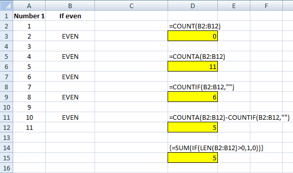
This will return a result of 5 which correctly returns the same result as when I combined the COUNTA and COUNTIF functions. Below is a summary of the results:

Excel spreadsheet showing a variety of count formulas.

If you liked this post on How to Count the Number of Cells With Text in Excel, please give this site a like on Facebook and also be sure to check out some of the many templates that we have available for download. You can also follow us on Twitter and YouTube.