Do you want to create a list of random numbers in Excel, but avoid repeating values? Below, I’ll cover how you can set that up to ensure that no number is shown more than once — all through just a single formula.
Start with the SEQUENCE function
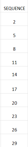
The first thing that’s necessary is to create a list of numbers to choose from. It needs to be in the form of an array, which can then be sorted. Using the SEQUENCE function, I can create an array which goes from 1 to 10 with the following formula:
=SEQUENCE(10,1)
The first argument specifies the rows to fill in, and the second one is the number of columns. If you wanted to start from the number 2 and jump by 3 values at a time, the formula would be as follows:
=SEQUENCE(10,1,2,3)
This produces the following, unsorted list:
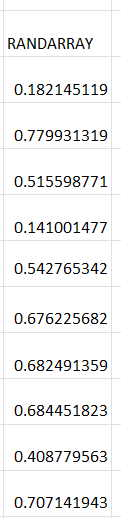
The next step is where the numbers get reordered. Another array of numbers needs to be created. This time, I’ll use the RANDARRAY function, since I want the array to be entirely random. I will again need to specify the number of rows and columns to fill in:
=RANDARRAY(10,1)
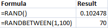
This produces a list of random numbers, similar to how the RAND function works. The only difference is that it creates a list for you:
Next, let’s combine these two formulas, within the SORTBY function. With the SORTBY function, you can specify the range you want to sort, and how you want it to be sorted. The complete formula is displayed as follows:
=SORTBY(SEQUENCE(10,1,2,3),RANDARRAY(10,1))
And this will now sort the sequence randomly. Here is the sorted and unsorted sequence, side by side:
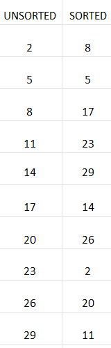
The column on the left, shows the unsorted values, as they have been created with the SEQUENCE function. The column to the right, however, has applied a random sort with the help of the RANDARRAY and SORTBY functions. The values are randomized and do not repeat. If you want to re-sort them, you just need to trigger a recalculation. This can be done by just pressing the delete key on any cell.
For this to work, both arrays have to be sized the same. In both functions, 10 rows and 1 column are used. However, if they are not the same size, the formula will produce an error. You could decide to have 1 row and 10 columns to display the values horizontally, with the following formula:
=SORTBY(SEQUENCE(1,10,2,3),RANDARRAY(1,10))
This will produce a randomized list which goes horizontally:

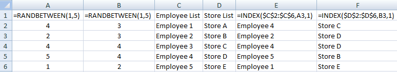
At this stage, you could use this random list as is or you could also combine it with a lookup function to extract a certain item based on a pre-defined value.
If you liked this post on How to Generate a List of Non-Repeating Random Numbers in Excel, please give this site a like on Facebook and also be sure to check out some of the many templates that we have available for download. You can also follow me on Twitter and YouTube. Also, please consider buying me a coffee if you find my website helpful and would like to support it.