FreeMathWorksheet

Free Math Worksheet and Template for Elementary School

If you have young kids who could use some math practice, I’ve got you covered. What’s great about Excel is that by using the random number generator, you can create an infinite number of worksheets for use over and over again. I’ve created a worksheet that includes addition, subtraction, multiplication, division, and other types of math work.

How the template works

Unlike other templates, you don’t need to enter any data for this one to work. It comes ready to go.
It’s simply a matter of removing or hiding whatever you don’t need. The template has 22 pages in total. There are pages that are for addition, subtraction, multiplication, division, patterns, rounding, greater than and equal comparisons, and ordering number in ascending and descending order.

If you view the workbook in Page Break Preview (this option is available from the View tab), this can help you decide where you want to hide/delete unneeded columns:
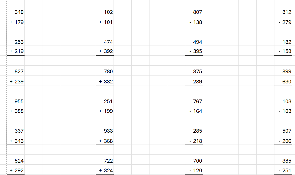
Math worksheet showing multiple pages.

For many of the values, they use the RANDBETWEEN function. If you’re comfortable with modifying the formulas, feel free to do so.
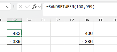
A formula using the RANDBETWEEN function.

In the example above, the formula finds a random number between 100 and 999. You could modify this to 1000 and 9999 if you wanted questions that are in the thousands.

The last two pages in this spreadsheet I’ve decided to covering a bit of everything. This can be helpful if you just want to print out a single double-sided page that can go over everything rather than printing out multiple pages.
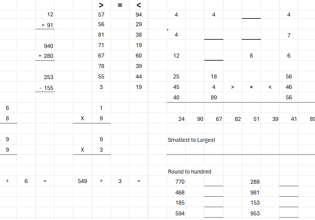
Math worksheets that cover many different types of questions.

Creating an endless number of worksheets!

What makes this template useful is that by simply triggering a recalculation, all the random numbers will change. So if you don’t like the numbers on a certain page, you can easily generate another set of numbers within a second. The easiest way to trigger a recalculation is to just select an empty cell on the sheet and press the delete key. Just make sure you’ve selected a cell that doesn’t contain a formula otherwise deleting it will remove it. If there’s nothing there, nothing gets deleted but the spreadsheet will recalculate.

Download the file

If you’d like to use the file, you can download it here. It’s completely free to use. I will add to it in the future and if you have any suggestions, please feel free to send them my way.


If you liked this Free Math Worksheet and Template for Elementary School, please give this site a like on Facebook and also be sure to check out some of the many templates that we have available for download. You can also follow me on Twitter and YouTube. Also, please consider buying me a coffee if you find my website helpful and would like to support it.

RAND Functions

Use Excel’s Random Number Generators to Populate Sample Data

Excel has random number generator functions which are useful if you need to test a template or create some sample / dummy data.

The RAND function returns a number between 0 and 1. You could multiply this by a factor of 10 or 100 to get a much larger number if you need it. Once you are happy with the data that has been populated then you will want to copy and paste it as values otherwise the numbers will change every time a recalculation occurs. This is true of any random number function in Excel.
Similarly, the RANDBETWEEN function will return a random  number between a range that you specify. In the below example I use 1 and 100:
RAND Functions
If I used the RAND function and just multiplied by 100 I could get similar results to RANDBETWEEN. The latter just saves you that extra step by being able to specify your parameters right in the formula. It allows you also to be more specific (say for example I wanted a random number between 1 and 35, the RANDBETWEEN function would certainly be easier to use)
If you do not like the random numbers you have generated, you can simply just hit the delete key on an empty cell and your random numbers will be regenerated. If you don’t want your numbers to change anymore then you will want to copy them and paste as values.
To use this to create sample data I am going to make two lists, one for employees, one for stores. From there, I can use the RANDBETWEEN function in conjunction with the INDEX function to extract values from the lists:
RANDBETWEEN Function
In columns A and B I am just using the RANDBETWEEN function to select a number between 1 and 5, as that is the number of different employees and stores I have listed in columns C and D. In columns E and F I use the INDEX function to extract from those lists using the random numbers generated in columns A and B.
I will break down the INDEX formula in column E a little bit here:
=INDEX($C$2:$C$6
In the first argument I am selecting my employee list since this is where I want the result to come from. I also lock the cells using the $ sign to ensure that as I copy the formula down that range is locked and will always reference C2:C6.
=INDEX($C$2:$C$6,A3
The second argument in the INDEX function is the row number from where I want to pull my value. Cell A3 is my first random value – which in this case is 4. This means that from the Employee List range (C2:C6) I want the value on the fourth row of that range – which is not row 4, it is row 5 since I start counting from the start of the range, which is on row 2. As I copy this formula down the row number will change to the corresponding value in column A. 
Because the lists only have one column you could actually stop here.
=INDEX($C$2:$C$6,A3, 1)
The last argument in the INDEX function is the column number. In this example I only have 1 column in my lists so the value is equal to 1. You could skip this argument and it will still work however it’s good habit to always enter the column number.
The above formula tells me to look at range C2:C6, and extract the value from the row that is referenced on A3 (which is 4), and from column 1. That point of intersection is Employee 4, since it is on the fourth line of that range, and in the first and only column.
If I copy the formula down a cell it will do the same except this time pull the value from the row referenced in cell A4 – this time it is 2. As a result, my result is Employee 2 since that value is on the second row of the range and again in the first column. 
Column F is the same formula as column E except this time it references the store list (column D) and the second RANDBETWEEN column (column B). This is just to show you how you might fill in multiple items. You wouldn’t want to use column A again otherwise you are guaranteed that the same row will be returned and you will always have Employee 4 tied to Store 4, and thus, not truly random combinations. 
In this example I have my lists, random numbers, and results all in the same area for illustrative purposes but they do not need to be even on the same sheet.