
Amortization schedules are essential tools for anyone managing a loan or mortgage, providing a clear breakdown of how payments are allocated towards interest and principal over the loan’s term. Typically, these schedules detail each payment’s date, the interest portion, the principal portion, and the remaining balance, offering borrowers insight into the precise cost of borrowing over time.
Creating an amortization schedule in Excel can be a time-consuming process, but with the help of some advanced payment functions, you can expedite the process and even eliminate the need for creating an entire amortization table.
Generating the key components of an amortization schedule
Whether you’re creating a full-blown amortization schedule or just want to calculate the balance at a future point in time, you’ll need to know the following values before you can begin:
- the loan value,
- the interest rate and compounding,
- the number of periods, and
- the start date of the loan
Suppose you have a $500,000 loan with a 5% interest rate, which is for a period of 10 years, and that payments are made on a monthly basis. Given this information, you can start by calculating the monthly payment amount. Here’s what the inputs would look like for the PMT function:
=PMT(0.05/12,10*12,-500000,0) = 5,303.28
This assumes compounding to be monthly, hence the need to divide the interest rate by 12. And the negative 500,000 balance tells the function that this is an amount owing and that it will reduce over time. The following argument, 0, is to signify that the future value is 0.
There is also an additional argument, for whether the payments are made at the beginning or the end of the period. The default is set to the end of the period. If payments are made at the beginning, then the final argument is set to 1. If the payment is at the start, then the payment value would change to $5,281.27, assuming all the other values remain the same. But for the purposes of these examples, we’ll assume payments are made at the end of the period.
Creating a calculator for specific month’s calculations
Now that you have all the necessary variables, including the payment amount, you can start to create the calculator.
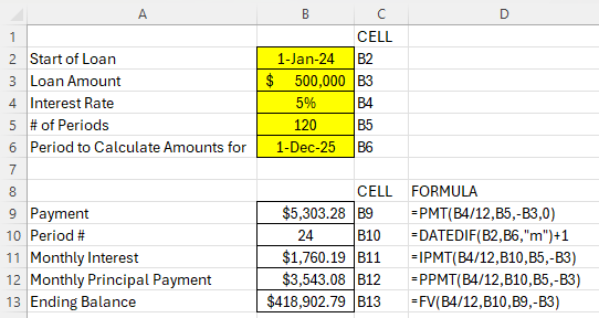
In this first case, we’ll look at how to calculate values for just a specific period. Let’s assume the loan’s start date is January 1, 2024. And let’s assume we want to calculate what the balance, interest, and principal payment amount will be for the month of Dec 2025.
How to calculate amortization amounts for a specific period:
1. Start with calculating the period number. One function that can help with this is the DATEDIF function. By using it, you can quickly calculate the difference between two time periods. Here’s how it would work in this example:
=DATEDIF(“1/1/2024″,”12/1/2025″,”m”) = 23
Two full years have not fully elapsed until we get to 1/1/2026. But since we want to calculate the values for the 24th month, we’ll need to add 1 to the equation. The formula to calculate the current period will be as follows:
=DATEDIF(“1/1/2024″,”12/1/2025″,”m”)+1
2. Calculate the interest payment for the period. To get the interest amount, use the IPMT function:
=IPMT(0.05/12,24,120,-500000) = 1,760.19
3. Calculate the principal amount paid down during the period. In this case, we can use the PPMT function. It is the same setup as the previous formula:
=PPMT(0.05/12,24,120,-500000) = 3,543.08
4. Calculate the ending value as of that period. Using the FV function, here’s the formula to get the ending balance as of the end of Dec 2025:
=FV(0.05/12,24,5303.28,-500000) = 418,902.68
By using these functions, you no longer need to make an entire amortization schedule. You can simply do a calculation for the period you need to sum up the values for. By creating inputs for the start of the loan, loan amount, interest rate, # of periods, and the period you want to calculate for, you can setup an amortization calculator as follows in Excel:
Calculate amortization values for a specific range
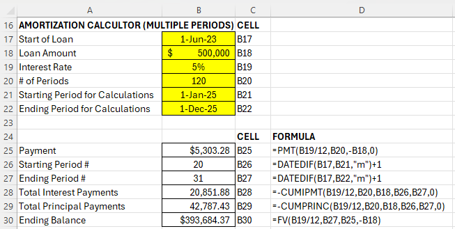
Suppose you wanted to calculate the interest and payment values for all the months in 2025. This can be a bit trickier since we aren’t calculating amounts for just a single period anymore. Instead, we need to get a range of values.
How to calculate amortization amounts for a specific multiple periods:
Step 1. Get the correct period numbers. Let’s assume the loan began on June 1, 2023. We need to get the starting period number, which is Jan. 1, 2025. This can be done with the DATEDIF function:
=DATEDIF(“6/1/2023″,”1/1/2025″,”m”)+1 = 20
This tells us that January is the 20th month of the loan. If January is the 20th month, then that also means if we add 11, that December will be the 31st month of the loan. Thus, our range of periods is 20 through 31. You could, however, use the DATEDIF function to do the calculation for that period as well.
Step 2. Calculate the interest payments for the year. Now that we know the periods we need to calculate the interest for, we can use the CUMIPMT function:
=-CUMIPMT(0.05/12,120,500000,20,31,0) = 20,851.88
The present value cannot be set to negative for the cumulative function, or else you will get an error. To adjust for this and avoid a negative value, simply add a dash before the function to ensure the result is flipped from a negative value to a positive one.
Step 3: Calculate the total of the principal payments made during the period. To calculate the principal paid during the period, we can use the CUMPRINC function. The inputs are the same as that of the cumulative interest payment calculation:
=-CUMPRINC(0.05/12,120,500000,20,31,0) = 42,787.43
Step 4. Get the ending period’s balance. Just as with the previous section, we can use the same FV calculation to get the ending balance. This time, it will be for period 31.
=FV(0.05/12,31,5303.28,-500000) = 393,684.23
Here is how the calculator could be setup to make these calculations based on a range.
You can download the amortization calculator I have created from these examples here.
If you liked this post on How to Create an Amortization Calculator in Excel, please give this site a like on Facebook and also be sure to check out some of the many templates that we have available for download. You can also follow us on Twitter and YouTube.