Microsoft Excel has been around for decades but Microsoft continues to roll out new features to enhance its software. Today, I’ll cover three recently released features that you need to know to be a more efficient Excel user.
1. A new shortcut that allows you to paste values
If you’re copying and pasting values in Excel and just want to paste the values, up until now, you’ve had to take the extra step of right-clicking and selecting values.
Although that doesn’t add a whole lot of time to the process, if there’s a more efficient way to do something, that’s what this website is all about. And the new way to copy as values requires just using the shortcut of CTRL+SHIFT+V when pasting. Whether you’re copying values from a website and don’t want to include formatting, or if you just want to copy a value from another cell and don’t want the formatting or formula, this new shortcut will be what you want to use.
2. The ability to search right from a menu
When Excel added the Ribbon, it grouped commands into different tabs. That can make it difficult to sometimes find commands because if you’re not on the right tab, you have to first navigate there before finding the command you want. One way around this has been to use the Quick Access Toolbar, where you can save your frequently used commands.
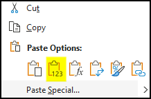
But even that isn’t ideal because you can’t add everything in there. The good news is that Excel has now added a search feature right into the default right-click menu. Simply right-click anywhere on your worksheet and you’ll now see a place to search for commands and functions:
3. An image function that allows you to pull in images from a URL
A new function that you can make use of in Excel will make it easier to load images into your spreadsheet. Rather than saving them and then uploading them into your workbook, all you need now is just the URL to the image you want to use. Then, within the new IMAGE function, just enter the URL in the first argument within quotation marks.
You can also specify an alt text and indicate whether you want the images to fit or fill the cell, or if you want to apply a custom height and width. In the below example, I use a URL that points to Netflix’s logo and have it fill in the cell. And as the cell expands, so too does the image:
Don’t have these options? Join the Office Insider program
These are the latest and greatest Excel features and so if you don’t have them and you’re using Microsoft 365, make sure you sign up for the Office Insider program. Through that program, you will have access to the newest features before the general public. Once joining, it may take a few days before you get the updates and start to see these features.
If you like this post on 3 New Excel Features You Need to Know in November 2022, please give this site a like on Facebook and also be sure to check out some of the many templates that we have available for download. You can also follow us on Twitter and YouTube.
Excel’s date and time functions make it easy to calculate the difference between two dates. And in this post, I’ll show you how you can calculate age in Excel. This can include a person’s age, or the interval between two dates. You can also break this difference into years, months, days, minutes, and seconds.
Use the YEARFRAC function to calculate the time in terms of fractions of years
One of the easiest ways to calculate age is by using the YEARFRAC function. As the name suggests, it will give you the fraction of a year. Suppose you wanted to calculate the difference between the start of the year 2000 and Christmas 2022. This is what your formula would look like:
=YEARFRAC("1/1/2000","12/25/2022")
Note that depending on your regional settings, you may need to enter date values in different formats. Alternatively, you could simply reference cells that contain date values so that you don’t need to do any hardcoding here.
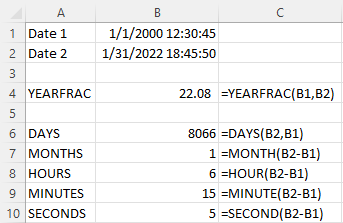
The above formula will return a value of 22.983. Since Christmas falls towards near the end of the year, the number is close to 23. If instead you choose Jan. 31, 2022 as the end date, then the formula would return a value of 22.083.
Use the TODAY function to make your formula dynamic
To calculate age so that it is always going to be up until today’s date, you can use the TODAY function. This avoids you having to enter the current date each time you want an up-to-date calculation. For example, if you wanted to calculate the fractional years between the start of 2000 and today, your formula would look like this:
=YEARFRAC("1/1/2000",TODAY())
The TODAY value will automatically update so you don’t need to do anything to trigger that calculation. Just by opening your workbook, Excel will pull in the current date value, and your formulas that contain the TODAY function will adjust accordingly.
Calculating month, day, hour differences
If you want to calculate the difference in months rather than fractions of years, there’s an easy way you can do that as well. Excel has a DATEDIF function that can make that process quick and easy. The logic is the same as with the earlier formula, but the main difference is that you enter “m” for a third argument, indicating month. Here’s the formula, using the same values as earlier:
=DATEDIF("1/1/2000","1/31/2022","m")
This formula gives a result of 264, which equates to 22 years. You’ll notice the drawback here is there are no fractions or rounding, just 264 months. If I adjust the end date to the start of February (“2/1/2022”), then it will return a value of 265 months. Until the month is complete, the formula won’t add the extra month, even if you’re selecting a date that’s nearly at the end (e.g. January 31).
One alternative you can make is to calculate the difference in days:
=DATEDIF("1/1/2000","1/31/2022","d")
This formula will return a value of 8,066. If you were to divide this by 365, you would get 22.09863. That’s the same answer I would get using the YEARFRAC function if I entered the last (optional) argument in that function to specify that I wanted to use 365 days for my calculation (the default calculation uses 360).
DATEDIF doesn’t have an argument that lets you calculate hours or minutes. However, with the number of days, you can approximate that by multiplying by hours. If you did want to get to that precise level of detail, you would need to create a separate formula for hours and minutes — and you would also need to ensure your date values included that level of detail to avoid approximation.
Using the HOUR, MINUTE, and SECOND functions, you can subtract the starting date from the ending date to arrive at a difference for each of those time calculations.. For these types of details, you should reference the cells as opposed to key in the hour, minute, and second values to ensure everything is entered correctly.
If you liked this post on How to Calculate Age in Excel, please give this site a like on Facebook and also be sure to check out some of the many templates that we have available for download. You can also follow us on Twitter and YouTube.
Switching back between Celsius and Fahrenheit can be cumbersome if you haven’t memorized the formula. There are multiple steps involved and you can easily make a mistake. And while you could use shortcuts to try and approximate roughly how it is, you can be more precise if you create a formula that you can use over and over again. If you’re using Excel, you can save yourself a lot of time as you can convert from Celsius to Fahrenheit (as well as in the other direction) using a formula which can compute the results in an instant.
What the formulas look like
The formula to convert from Fahrenheit to Celsius is as follows:
C = 5/9 x (F-32)
And this is the formula for the reverse:
F = (C x 9/5) + 32
You could set these formulas up in Excel just with simple arithmetic. The downside of that is then you have to create multiple formulas (one for Celsius and one for Fahrenheit), or even set up a small template just to do that. But Excel makes it even easier do to that as it has a function which can save you all those steps — it even knows the formula so you don’t have to memorize it!
Using the CONVERT Function
There’s convenient function right within Excel that can convert between different measurement values, called CONVERT. As the name suggests, it can convert values for you. It takes three inputs: the current value, what unit you’re converting from, and the unit you want to convert to. The formula to convert Fahrenheit into Celsius is as follows:
=CONVERT(A1,”F”,”C”)
Where A1 is the value in Fahrenheit. To do the reverse, you just need to flip the symbols:
=CONVERT(A1,”C”,”F”)
The key thing you just have to remember is that the unit you’re converting from comes first, followed by the unit you’re converting to. Those values need to be in quotes so that Excel reads them correctly as a text values.
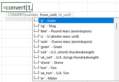
This function is a lot more powerful and there are even more items you can convert between, simply look through the list of possibilities as you are entering the arguments.
You can flip between date values, measurements, weights, and many other things. The CONVERT function is much more powerful and converting between Celsius and Fahrenheit is just one of the many things it can do.
If you like this post on How to Convert Celsius to Fahrenheit Using an Excel Formula, please give this site a like on Facebook and also be sure to check out some of the many templates that we have available for download. You can also follow us on Twitter and YouTube.
Do you want to calculate how quickly it will take for something to double in value? In this post, I’ll show you how to calculate that using the doubling time formula. By utilizing variables, it can also be easily updated in Excel to factor in different growth rates, making it easy to do what-if calculations.
What is the doubling time formula?
The doubling time formula utilizes logarithms and takes an assumed growth rate to determine how long it will take for a value to double in value. For example, if your investment were to rise at a rate of 10% per year for 10 years, it would be worth roughly 2.59 times what it is now. But rather than doing trial and error to try and determine exactly at what point it will double in value, you can use a formula to do that for you.
In essence, all the doubling time formula involves is taking the logarithm of the change in value you’re trying to get to (e.g. 2) and dividing that by the logarithm of the current growth rate plus 1 (e.g. 1 + 0.1 = 1.1). By doing this calculation, you get an answer of 7.27 for this example. You can plug that into the following formula to check:
1.1^7.27
And the result will 1.9995. The more decimal places you keep in the above calculation, the closer you will get to precisely 2. This formula can also be adapted if you want to calculate how long it will take to triple, or quadruple. In those cases, you can just change the numerator so that instead of taking log 2, you’re taking log 3 or log 4, if you want to calculate tripling or quadrupling time, respectively.
Setting up the formula in Excel
As you can see, this isn’t a terribly complex formula. The key is really just using logarithmic functions in Excel. And whether you use a natural log or not doesn’t matter, your results will be the same. You can use the LOG function for these purposes. In Excel, the earlier formula would be calculated as follows:
=LOG(2)/LOG(1.1)
To make it more versatile, I’ll also add some variables here. One for the current growth rate, and one for the target growth (this is where you can specify if you want to double, triple, quadruple, etc.). Here’s how that looks:
A value of 2 will read as 200% in Excel. The formula to calculate the years to double will simply need to be adjusted to factor in for these variables, which I’ve named TargetGrowth and GrowthRate in my file:
=LOG(TargetGrowth)/LOG(1+GrowthRate)
By utilizing these variables, I can now easily update my calculations.
Creating a LAMBDA function to make it even easier
Another thing you can do is to create your own LAMBDA function. If you’re on the latest version of Excel, these are custom functions you can ease, without the need to even set up a template and separate cells. All this involves is going to the Name Manager in Excel as if you were creating a new named range (the long way). Except when you create it, the name you’re assigning is the name of the function. And rather than referencing cells, you’re entering in a formula.
This particular function should contain two variables, one for the current growth rate, and one for the target. It will then plug them into the formula I referenced above. Here’s what the formula will need to look like within the Name Manager:
You’ll notice it needs the LAMBDA prefix so that Excel knows to treat this differently. Here’s how it looks within the Name Manager:
I called it DoublingTime even though it can do more than just calculate that. You can of course call it whatever you prefer. Now, this formula can be used in Excel to do the exact same calculation as above, without the need for extra cells:
You’ll notice here I’m just entering in raw values as opposed to percentages. This is just because of how I structured the formula and to keep it as simple as possible.
If you liked this post on Calculating the Doubling Time Formula in Excel Functions, please give this site a like on Facebook and also be sure to check out some of the many templates that we have available for download. You can also follow us on Twitter and YouTube.
A VLOOKUP function is simple: you enter criteria and select a range that it should extract values from. However, there are multiple reasons why your VLOOKUP cannot find the correct value. Below are seven common reasons your formula may not be working as you expect it to.
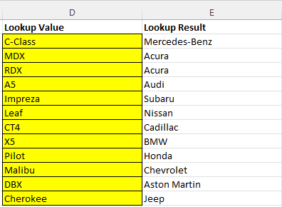
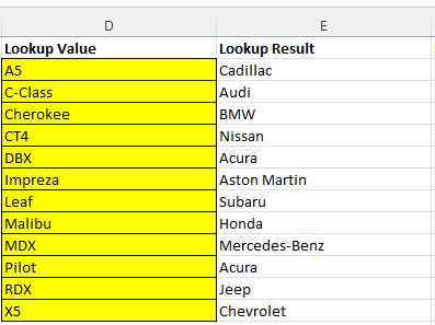
In this example, I’m going to use the following list of automobile makes and models:
I’m going to use a lookup formula to find a model and identify the make. The model and make values are in columns A and B on my sheet, respectively. And my lookup value is cell D2. The correct formula would be as follows:
=VLOOKUP(D2,A:B,2,false)
There are four arguments, and here are some of the common ways you could mess this formula up:
1. You didn’t enter the correct range
=VLOOKUP(D2,A1:B100,2,false)
A common error is that you enter a range that doesn’t cover the area that you need. For example, in the above example, the formula goes only to row 100. But if the value you want is on row 101, the lookup formula won’t work and you’ll get an #N/A error.
Another issue could be the following:
=VLOOKUP(D2,B:C,2,false)
In this situation, the formula is starting at column B but the model list is in column A. That all but guarantees that it won’t find the right value. In a VLOOKUP formula, you are looking up the leftmost column in your range. If the model values are in column A, that’s where the formula needs to start from. In the above formula, it will be looking for the values in column B, which isn’t correct.
2. You are extracting values from the wrong column
=VLOOKUP(D2,A:B,3,false)
The range is fixed in this situation but the problem here is that you’re looking for the value in the third column. There are only two that are in the formula. In this instance, you’ll get an error because you’re trying to access a value that’s outside of the range you provided.
=VLOOKUP(D2,A:B,1,false)
The range is correct but here the problem is now you’re referencing the first column. Although you’ll get a value, it will be the same one you input, since the formula is looking at column 1.
One of the common issues with lookup formulas is that people are referencing column numbers that can change over time as they expand their data set. Those numbers won’t automatically adjust when you insert new columns.
There are a couple of workarounds for this. One is to use convert your data set to a table and reference an actual table column. Another is to use the MATCH function to find the column number that you’re looking for. Alternatively, you could use a combination of INDEX & MATCH.
3. You misspelled the value you’re looking up
One of the easier mistakes to spot is when you’ve misspelled the name of what you’re looking up. If in your lookup formula you want to find “Accord” but instead type in “Accorrd” then you’ll end up with another #N/A error. However, if you have a data set where the lookup values could be similar, the danger there is that you could potentially not get an error and instead return the value that relates to a different lookup value. The best way around this is to avoid hardcoding your lookup values. That way, it can be easier to spot errors and it’ll be easier to adjust them.
The reverse is also a problem: if your lookup column contains a misspelling. In that situation, even though the value you’ve looked up is spelled correctly, your lookup could still fail.
4. Your value has extra spaces
One of the trickiest mistakes is where your data isn’t misspelled but contains an extra space somewhere. Just by looking at a cell, you may be able to spot when there’s a leading space. But if there’s a trailing space, that’s tougher and you may not notice until you actually go in and try to edit the value. Whether it’s an extra space or the value is misspelled, that can impact your ability to find a match.
The way to check your data is by using the RIGHT function (or the LEFT function if you want to confirm the first character). If you enter the following formula to reference D2 (the lookup value), it will return the last character in the cell:
=RIGHT(D2)
If it returns a blank value, you’ve found your problem. Similarly, you can use this formula on your lookup list to see if any values have extra spaces. This is something you’ll want to do before creating your lookup formula. Making sure your data is good to go and clean with no trailing spaces can save you from encountering these issues later on.
Removing blank spaces can be easy but sometimes it can be tricky as not all blank values are the same.
5. Your value is reading as the wrong data type
In this example, the lookup is a text value. However, one potential error happens when you’re looking up a number that is stored as text. That can also result in no match being found. A good way to spot this error is to see if your data aligns to the left or the right by default. If you have no formatting applied, text should align to the left, while numbers will shift to the right. Another way you can check if something is reading as text or a number is to use the ISTEXT function. To convert a number stored as text into a number, multiply it by 1.
6. You search for an approximate match when you want an exact match
In most cases, you’ll probably want an exact match from your lookup formula (i.e. you’ll set the last argument to FALSE). The one exception I’ve found to be most useful is when you’re dealing with numbers and ranges. With tax brackets, for example, you’d be looking to see what range a value falls into versus an exact match.
In error #1 on this list, if you set the last argument to TRUE and looked for an approximate match, you would get a result, it just may not be the one you were hoping for.
7. You’ve sorted your formulas and they’re not correct anymore
A frustrating problem can be when you’ve entered your formula correctly but when you sort your formulas, they’re now referencing the wrong cells. In this case, you’re dealing with multiple lookups at a time. For example:
The lookup values are correct but if they get re-sorted, they’re now referencing the wrong values and the lookup results are incorrect:
After sorting column D in ascending order, the formula is incorrectly saying that Acura makes the Pilot and that there’s a BMW Cherokee. Here’s what the formula looks like in cell E2 before sorting:
=VLOOKUP(Sheet1!D2,A:B,2,FALSE)
The error is in the sheet reference. Since it’s including Sheet1!D2 instead of just D2, the value isn’t automatically updating when resorting. Excel automatically inserts the sheet referencing if you’re editing a formula and jumping from one sheet to another. The formula is locking that value in place, even when you sort. Getting rid of the sheet references fixes the error.
If you liked this post on 7 Reasons Why VLOOKUP Cannot Find the Right Value, please give this site a like on Facebook and also be sure to check out some of the many templates that we have available for download. You can also follow us on Twitter and YouTube.
Parsing data in Excel can be complicated, using a combination of functions ranging from LEFT, RIGHT, MID, and FIND. However, with the help of a few new functions that are available in Excel, the process is a whole lot easier for users. In this post, I’ll look at how you could parse out a date that is formatted as text using the new functions and comparing that with how you might have done it using the old functions.
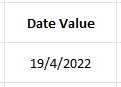
In this example, I’m going to try parse out the numbers I need to convert the following value, which is reading as text:
This date is April 19, 2022. But because my regional settings are set to month/day/year this value doesn’t compute properly since it would be looking for a 19th month.
Pulling the day value (data before the delimiter)
The old method
The first number in the date value above relates to the day of the month. Using the LEFT function in Excel, you could use something like this:
=LEFT(X,2)
Where X is the cell value. That will pull the first two characters in the string. But in some cases there might only be one day for the date. And for that reason, I’m not going to hardcode the number of characters. The best approach (under the old method) is by using the FIND function to locate where the delimiter (“/”) is. The more versatile formula would look as follows:
=LEFT(X,FIND("/",X,1)-1)
The new method
One of Excel’s new text functions is called TEXTBEFORE. And as the name suggests, it will extract all the text that comes before a delimiter. Without needing the FIND function, I can simply do this to extract the day value:
=TEXTBEFORE(X,"/")
Pulling the year value (data after the delimiter)
The old method
To grab the year in the date I could cheat and use the RIGHT function and just grab the last four numbers. But that wouldn’t be flexible enough in the event that I might have 2 digits instead of 4 as the year. This can get messy as now I have to use multiple FIND functions in order to determine the length. The key is to take the length of the function and subtract from that the position of the second delimiter. Here’s what that looks like:
=RIGHT(X,LEN(X)-FIND("/",X,FIND("/",X,1)+1))
The nested FIND functions can get a bit complicated. Here you’ll see even more efficiency with Excel’s new functions.
The new method
The TEXTAFTER function can greatly simplify this action because you can specify after which delimiter you want to pull the characters; there is no need to have nested functions with this:
=TEXTAFTER(X,"/",2)
In this formula, the characters after the second “/” will be extracted. Note: both the TEXTBEFORE and TEXTAFTER functions allow you to specify the instance of the delimiter (i.e. it doesn’t always need to be the first one).
Pulling the month value (data between delimiters)
The old method
The most challenging part of this process is undoubtedly to pull the data between delimiters. In this example, I’ll need to use the MID function and use nested FIND functions to determine the space in-between the delimiters. It’s an ugly formula if you don’t rely on hardcoding:
That’s four FIND functions in one formula. You can quickly see how parsing out this information can be a challenge. But with the new Excel functions, it’s much easier to do this.
The new method
There isn’t a new function that specifically pulls the values between delimiters. But by using both the TEXTAFTER and TEXTBEFORE functions, you can do exactly that. Let’s start with just grabbing everything after the first delimiter:
TEXTAFTER(X,"/")
This will give us the following result: 4/2022. Obviously that’s not what I want. But now, I can nest this within the TEXTBEFORE function, and grab the value before that other “/” with the following formula:
=TEXTBEFORE(TEXTAFTER(X,"/"),"/")
We are still dealing with a nested function here, but this is no doubt easier than all those FIND functions under the old method.
Using an array function
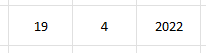
Another option that you can use is to extract all the values between the delimiters using the TEXTSPLIT function. Simply enter the following formula:
=TEXTSPLIT(X,"/")
Then the values will be extracted into three cells, one for the day, month, and year:
The benefit of this approach is you can quickly pull everything from the cell you’re parsing data from.
Regardless of which option you choose, Excel has given its users some new tools that can make the parsing much easier and less complicated than it was before.
If you liked this post on Excel’s New Text Functions, please give this site a like on Facebook and also be sure to check out some of the many templates that we have available for download. You can also follow us on Twitter and YouTube.
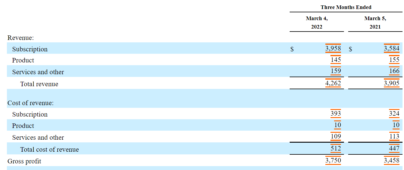
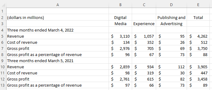
If you want to download a company’s financial statements or data, the easiest place is often straight from the source: the Securities & Exchange Commission (SEC). You can download financials in Excel format if there is an interactive option within the SEC filing, but that won’t give you all the tables contained in an earnings report. In this example, I’m going to use Adobe’s most recent earnings report to show you how to get a table into Excel
Downloading the data
Adobe’s earnings report is found here, with the following financials on page 4:
Copying it into Excel
Copy the table and then go to paste it data into Excel. But when you right-click in Excel, make sure to select the option to paste it so it matches the formatting on the sheet, as shown below:
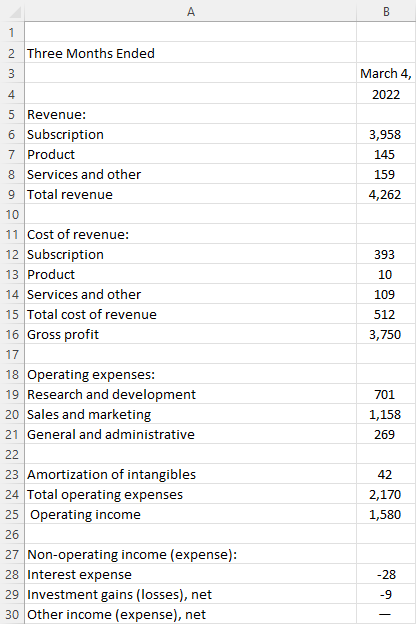
Now, the data pastes without any of the colors and formatting onto my Input sheet:
If when you paste it doesn’t show up like this and it looks like just a few lines, re-try copying the data. It may help not to include the header that says “three months ended” and simply start copying from the first line item (“revenue” in the above example”) to ensure that Excel picks it up as a table.
Formatting the data
It looks pretty good except that I have many extra columns. And numbers that have dollar signs have been pushed out by one column. What I will do here is create a template in a separate sheet that will automatically pull in what is needed. The new tab, called Output, will be where I create my formulas. My assumption is that the spacing will be consistent and that the current period values are in columns D and E, and the ones from the prior-year period are in columns J and K.
Starting in cell A1, I’ll create a simple formula that checks if the same value on the other sheet is blank. If it isn’t, then it will pull in the value, otherwise, it will remain blank:
=IF(Input!A1="","",Input!A1)
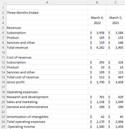
I will do the same thing for column B, except this time I am looking at values from the Input tab in column D. And I will need to adjust for if there is a $ sign. If there is, I need to pull the value from column E instead. Here’s what that formula looks like:
That gets me a bit closer to where I want to get to:
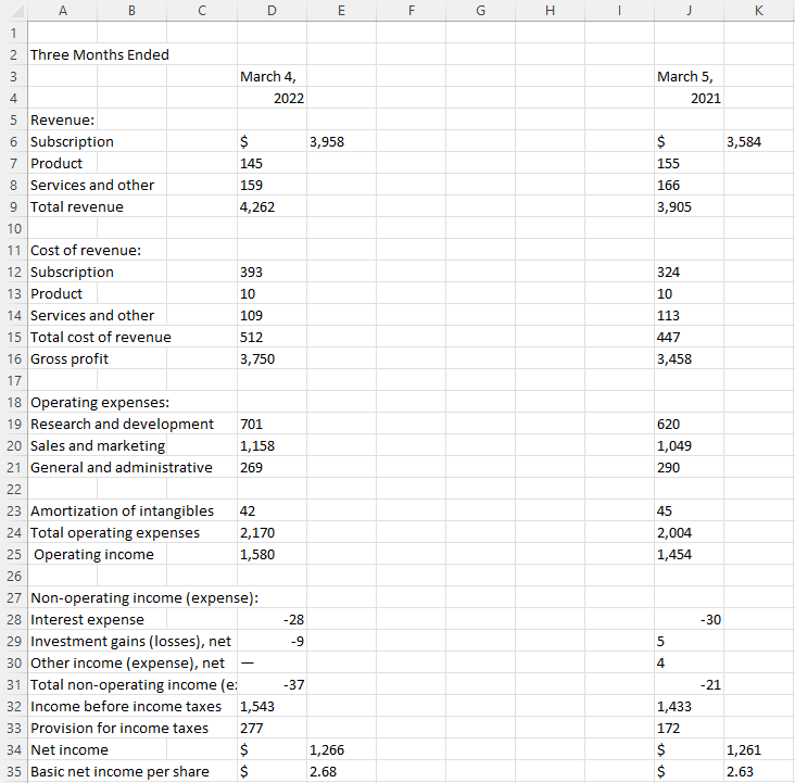
There are still a couple of issues. The first is that on row 30, there is a symbol that isn’t a dash that I need to remove. This is character code #151. And there’s also a trailing blank space behind the numbers that needs to be removed. This isn’t your ordinary blank space and it is character code #160. I need a couple of SUBSTITUTE functions to remove those character codes:
For character 151, I want to replace this with a 0 value since that’s what the symbol is in place of. Next, I need to convert these values to numbers. I can do this by multiplying them by a factor of 1. I’m going to use the IFERROR function as well so that in case it’s text, it will return the original value in column D. Here’s my completed formula:
Now, I can repeat this formula in the adjacent column. Except this time instead of referencing D and E, I’ll refer to columns J and K. Now, my output tab looks as follows, after applying some formatting to it:
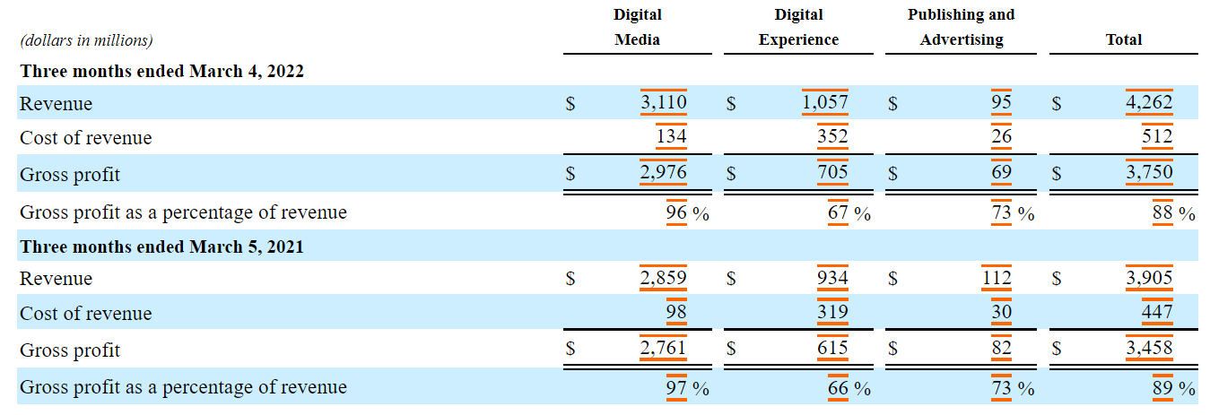
This can be re-used over for other tables in an SEC report, as they generally follow the same pattern. For example, this is Adobe’s table showing sales by segment:
By dropping this into my Input tab, this is what my Outputnow shows:
All that I needed to do was to copy the formulas and just adjust the columns they referenced on the Inputtab. If you’d like to use the file I’ve created for your own use, you can download it for free, from here.
If you liked this post on How to Convert a Table From an SEC Report Into Excel, please give this site a like on Facebook and also be sure to check out some of the many templates that we have available for download. You can also follow us on Twitter and YouTube.
Do you want to calculate how long a team’s winning streak is, or how many cells in a row meet certain criteria? In this post, I’ll show you how you can calculate streaks in Excel. Unlike a simple count function, this will require being able to reset your count and go back to zero. I’ll show how this can be done using an easy approach that involves a helper column, and a more challenging way that doesn’t require one.
The easy way to calculate streaks
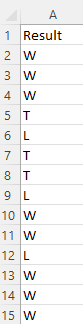
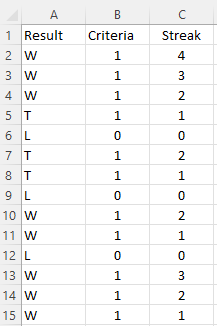
Here are some results, showing wins (W), losses (L), and ties (T).
The helper column I’m going to create will evaluate the criteria. And the criteria, in this case, will be whether the result is a win. For this, all that’s required is a simple IF statement checking if the value is a W:
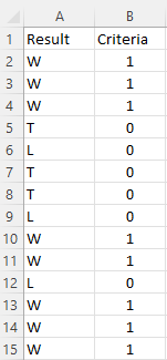
=IF(A2="W",1,0)
If the result is a W, the formula will return a value of 1, otherwise, it will be 0:
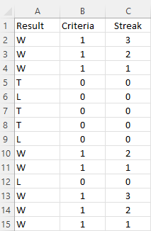
Next to that column, I will create another one for the actual streak. This formula will look at the criteria column, and if it equals 0, then the streak is 0. If it’s a value of 1, then it will add on to the previous value in the streak column, and thus, add on to it. The formula is as follows:
=IF(B2=0,0,B2+C3)
And that results in the following calculations:
The assumption here is that the earlier results are at the bottom and the most recent games are at the top.
If you wanted to calculate how many games were either won or tied in a row, and thus, an undefeated streak, all you need to do here is to adjust the criteria column. The updated formula would be this:
=IF(OR(A2="W",A2="T"),1,0)
And now the streak values change:
The difficult approach, without helper columns
If you don’t want to use a helper column, calculating streaks is a bit more challenging. You will be using an IF function and checking for criteria, but this time you’ll need to always adjust your starting point (i.e where the streak is 0). And that will need to be within a SUM function to ensure that the values are added. The key to making this work is using the INDIRECT function so that you have control over the exact range you want to include.
Inside that function, I’ll start with column A and use the current row the cell is on, which can be done using the ROW function. Here’s how it starts:
INDIRECT("A"&ROW(B2)&":A"
B2 reflects the first cell in the streak calculation, and it will return a value of 2. The last cell needs to be the last time the streak was broken — when the team recorded a loss. This involves using the MATCH function and searching for an “L”. That formula is as follows:
MATCH("L",INDIRECT("A"&ROW(B2)&":A15"),0)
Here again, I use the ROW function and as my ending cell, I put A15, which is the last cell in the range. This could be adjusted to use a MAX function to make it variable. Since the MATCH function will return a number corresponding to its position within the range (e.g. it won’t return the actual row), I will adjust for the row number immediately above the first cell to be searched. In this case, since I’m searching cells A2:A15, I need to add 1 to ensure I get the row number and adjust for the fact that the MATCH function doesn’t begin from the very first row. I will add all this together into my earlier formula:
The one last adjustment that’s necessary is to account for if there is no loss found and the team starts on a winning streak. For this, I’ll add an IFERROR function just before the MATCH function so that if it evaluates to a 0 (after adding the 1), then it will default to the last row (15):
Given how complex this formula is, it can get messy if you create too many conditions in it. And if you do have multiple criteria you’re dealing with, then the first approach may be the more practical one to use in that case.
If you liked this post on How to Calculate Streaks in Excel, please give this site a like on Facebook and also be sure to check out some of the many templates that we have available for download. You can also follow us on Twitter and YouTube.
In Excel, you can create quick and easy visuals with only a formula. You don’t need to insert charts or worry about if they are set up correctly. In this post, I’ll show you how you can quickly create both bar and column charts.
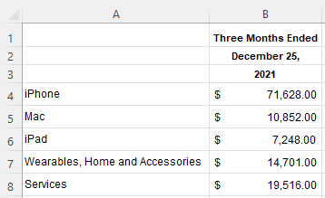
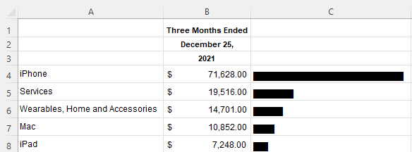
For this example, I’m going to use data from Apple’s most recent earnings report, to see the split between sales of its different categories. Here’s what the data looks like from its most recent filing:
To create a simple bar chart, I’m going to use the REPT function, which allows me to repeat text. The character I’m going to repeat is the “|” line, which on most keyboards is the button above the enter key. Holding shift and that key should give you that line. The number of times I want to repeat the character will be the value in column B. But because it’s too large, I’m going to divide it by a factor of 100. Here’s how that formula will look:
=REPT("|",B4/1000)
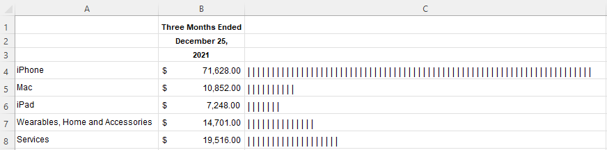
If I copy this down, my bar chart remains a work in progress:
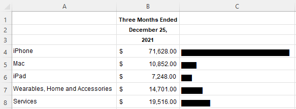
One way to make this look like more of a bar chart is by changing the font. In column C, I’m going to change it to Britannic Bold. And now, this looks like a proper bar chart:
If I sort the values from largest to smallest, then it’s easier to see the progression:
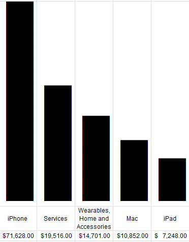
This is good, but this is also still a bar chart. To convert this into a column chart, I need to make a couple of changes. The first thing is I need to arrange the data differently so that the fields and the values are going horizontally rather than vertically. To do this, you can just transpose the data. You can do this using the TRANSPOSE function. Now, my data is better suited for a column chart:
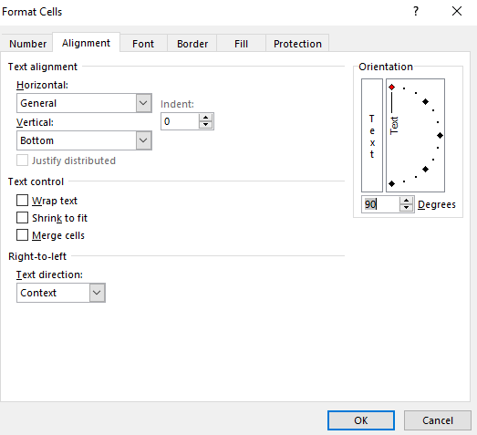
Now, I’ll add back the REPT function and use the same font. Except for this time, I will modify the cells so that the alignment is vertical:
Now, after compressing the columns, I have a column chart set up:
Here’s a quick video showing the steps:
If you liked this post on How to Create Column Charts in Excel With Just a Formula, please give this site a like on Facebook and also be sure to check out some of the many templates that we have available for download. You can also follow us on Twitter and YouTube.
Did you know that you can group numbers in Excel using tags? By just listing all the categories an item should belong to, you can make it easier to group them. In this post, I’ll show you how you can use tags in Excel to efficiently summarize different categories.
Creating tags
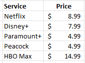
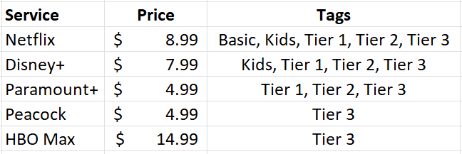
Suppose you wanted to list all the possible streaming services you might subscribe to. You might have a list that looks something like this:
This is fine if you want to compare them or even tally them all up. But what if you wanted to look at different scenarios, such as what if you select some of these services, but not all of them? This is where tags can be really helpful. Let’s say I want to create the following categories:
Basic
Kids
Tier 1
Tier 2
Tier 3
Each category will have a different mix of services. Here’s how I can use tags to make that happen. I’ll create another column next to the price where I specify all the categories a service will fall under:
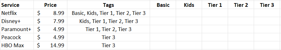
In the above example, Netflix is included in every package but HBO Max is only included in Tier 3. Next, what I’m going to do is create columns for each one of these tags, such as follows:
Without using tags, you might be tempted to put a checkmark to determine which service belongs in which category. But that’s not necessary here. Instead, I’m going to use a function to determine whether to pull in the price or not.
Using a formula to determine if a tag is found
The key to making this work is the SEARCH function. This will look within the tag values to see if there is a match. If there is, then the price will be populated within the corresponding category. To check if the ‘basic’ keyword is found within the tags related to Netflix (assume this is cell C2), this is how that formula would look:
=SEARCH(“basic”,C2,1)
This will return a value of 1, indicating that the term is found at the very start of the string. If you use the function to look for the word ‘kids’ then it would return a value of 8 as that comes after ‘basic in my example.’ Of key importance here is that there is a number. If there isn’t a number and instead there is an error, that means that the tag wasn’t found. I will adjust the formula as follows to check if there is a number:
=ISNUMBER(SEARCH(“basic”,C2,1))
This will return a value of either TRUE or FALSE. But the formula needs to go further than just identifying if the tag was found. It needs to pull in the corresponding value. To do this, I’ll need an IF statement to extract the value from column B:
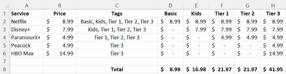
=IF(ISNUMBER(SEARCH(“basic”,C2,1)),B2,0)
By freezing the formulas and copying this across the other categories, this formula will now allow me to pull in the amounts correctly based on the tags:
But let’s say you don’t even want to do this, you just want to quickly group the totals without these extra columns. You can also do that with the help of tags.
Summarizing the totals by category
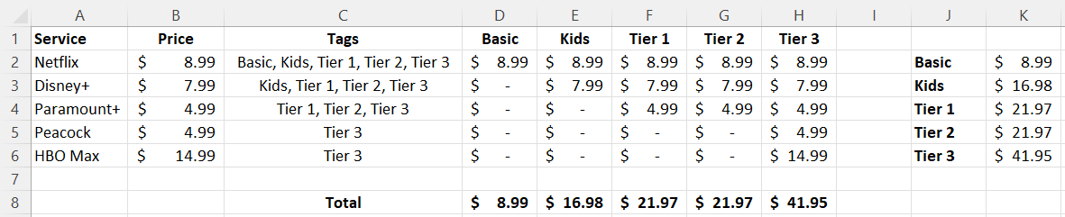
You don’t need to create a column for each group if you don’t want to. You summarize the total in just an array formula. Simply use the formula referenced earlier and include it within a SUM function, while referencing the entire range:
This is the same logic as before, except this time the values will be totaled together. On older versions of Excel, you may need to use CTRL+SHIFT+ENTER after entering this formula for it to correctly compute as an array. But if you’re using a newer version, you don’t need to. If you copy the formula to the other categories, you’ll be able to sum the values by without the need for additional columns:
If you liked this post on Using Tags in Excel, please give this site a like on Facebook and also be sure to check out some of the many templates that we have available for download. You can also follow us on Twitter and YouTube.