In Excel, IF statements give you way to handle multiple scenarios. You can determine which result to return based on another value or input that a user makes. A common example is where a cell contains no value. You can create a formula to say if the value is blank, you return a result that is blank. And if it isn’t blank, you can perform a calculation. IF statements work similarly in Power Query although you can’t enter them in cells. Below, I’ll show you how you can create a conditional IF statement in Power Query and how you can use it in your data set.
In this example, I’m going to use data from the data.gov website on the Tuition Assistance Program. You can download the CSV data from here if you want to follow along.
Getting the data into Power Query
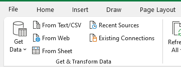
Once you have downloaded the data, the first step is to pull it into Power Query. For that step, just click anywhere on the data set and under the Data tab, click on the option to get data From Sheet:
The data is fine in the shape that it is right away so there is no need to make any changes when loading it into Power Query.
Creating a Conditional Column in Power Query
Suppose we wanted to just differentiate the data between whether the funding is related to the private sector or the public. You could do a pivot table but if you want to just have a column to pull in those amounts separately, you can create a conditional column. A conditional column works like an IF statement, only it is easier to set up.
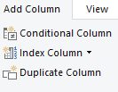
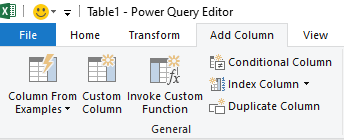
One thing to remember with Power Query is if you want to just alter the current column, you want to stay on the Transform tab. But if you want to create a brand new column — which is what I’ll be doing in this example — you want to go onto the Add Column tab at the top:

Once you are on the Add Column section, you will see an option for a Conditional Column right below it:
Click on that button, and then you will see the following window:
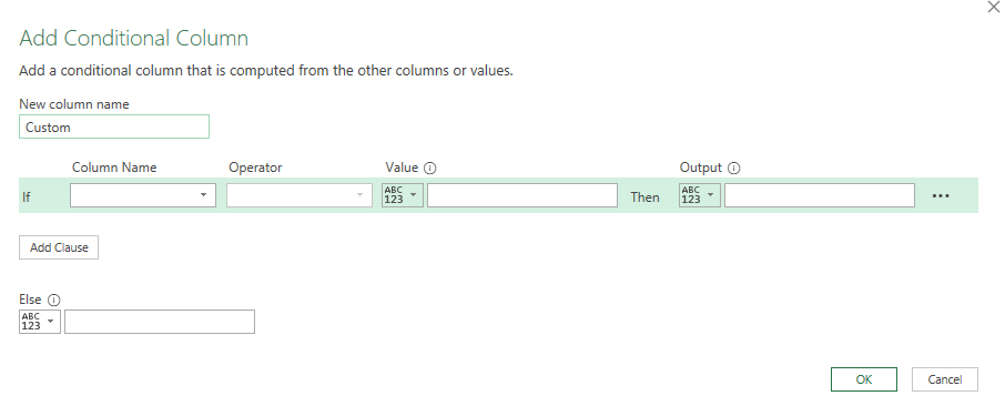
For the column name at the top, I will call it Private Funding, since that is what I want to calculate. And the criteria is simple: I’m going to set it so that if the Sector Type column is equal to PRIVATE (this is case-sensitive in Power Query), then the output will be the TAP Recipient Dollars column. Otherwise, I want the value to be zero. Here is what that looks like:
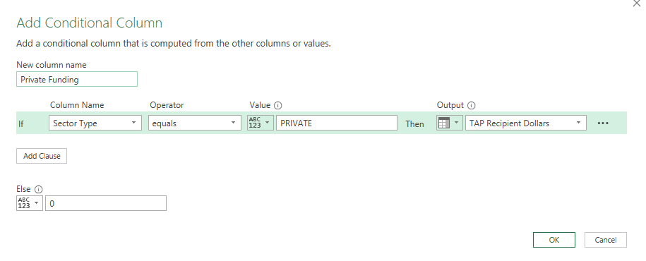
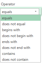
You’ll notice that on the output, value, and else fields, there is a down arrow. Clicking on this will allow you to switch between a column or a value. You can specify if you want to enter a value or reference a column. In this case, I want to reference an entire column if the criteria is met. And if it isn’t, I want to set it to a value — zero. For the operator, you also don’t need to look for an exact match, that too can give you various options:
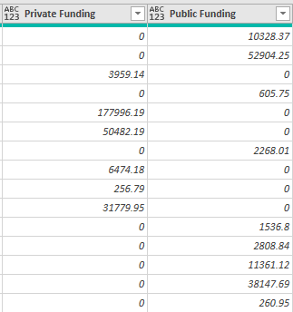
Once that is set up, I have a column called Private Funding in Power Query that is equal to the TAP Recipient Dollars if it is Private funding only. Otherwise, it is set to 0:

Now, I can repeat these steps for Public Funding and will now have a value in either private or public funding:
You may think this is a bit redundant but it saves having to create a pivot table if I wanted to do a summary (or a SUMIF function). One of the great things about Power Query is when I no longer need a column, I can just delete it. If I right-click on the original Sector Type column, there is an option to Remove from the shortcut menu:
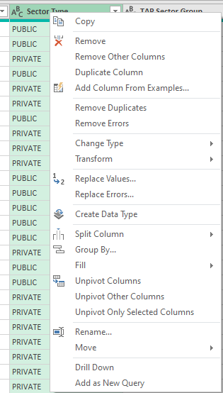
This doesn’t impact my table because Power Query saves the steps I take and each time repeats the same order. This way it is safe to remove the unnecessary tab and avoid having redundant data that isn’t needed anymore.
Using the conditional column option is easy but if you want something more versatile to possibly include other Power Query functions, you can also use the Custom Column button, which I’ll cover next.
Creating an IF Statement Using a Custom Column
The option to create a Custom Column is also under the Add Column section:
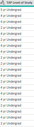
In this example, I will create a conditional column to look at if the TAP Level of Study column indicates at least a 4-year degree. By looking at the values there, we can see that the years are indicated in the first number:
If this was in a spreadsheet, I could just use the LEFT function to extract the first number. But in Power Query, I’m going to do it a little differently. Instead of the LEFT function, I am going to use the Text.Start function (these are also case-sensitive), which works the same way:
Text.Start([TAP Level of Study],1)
In this formula, I’m selecting the field, TAP Level of Study, and extracting just the first character from that. However, I still need to convert this into a number if I want to evaluate it as one. Next, I need to enclose this within the Number.FromText function. My formula looks like this:
Number.FromText(Text.Start([TAP Level of Study],1))
The next step is to evaluate it to see if the value returned is greater than or equal to 4:
Number.FromText(Text.Start([TAP Level of Study],1)) >= 4
If I am content with just getting back a series of TRUE or FALSE values, then I can stop here. But if I want to customize the values to say ‘YES’ or ‘NO’ then I will need to add to this formula by adding an ‘if’ statement at the beginning. I will also need to use the ‘then’ and ‘else’ keywords to tell Power Query what I want the results to be:
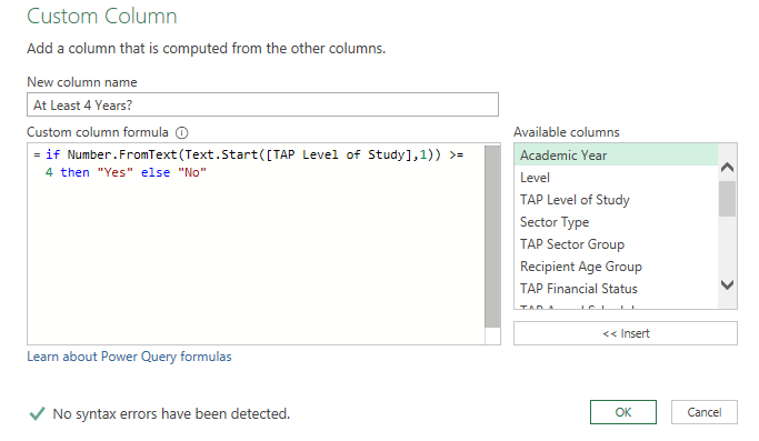
if Number.FromText(Text.Start([TAP Level of Study],1)) >= 4 then “Yes” else “No”
This is how it looks in the Power Query Custom Column window:
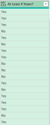
As you can see, going through the Custom Column approach will give you more flexibility as to what you can do with your conditional statements. While the Conditional Column is easy to use, it isn’t as flexible as you might need it to be. Now, when I click OK to create this column, I know have values that show either ‘Yes’ or ‘No’:
If you are looking for other Power Query functions, you can check out this page.
If you liked this post on How to Make a Conditional If Statement in Power Query, please give this site a like on Facebook and also be sure to check out some of the many templates that we have available for download. You can also follow us on Twitter and YouTube.